Dielectric function: job_eps
⚠️ Tool consolidation (2026-06) — The dielectric-function driver is now
job_eps(with--lcffor local-field correction,--decomposefor interband / intraband split). The legacyepsPP0/eps_lmfh/epsPP_lmfh/epsPP_lmfh_intrawrappers have moved toSRC/exec_legacy/and are no longer installed to~/bin.TOML migration (2026-05) —
job_epsreadsctrlg.<sname>.toml+PB.<sname>.toml. Convert legacyctrl.<sname>/GWinputdirectories withLegacy2toml.py <sname>. See TOML migration and worked examples in Samples/EPS/ —EPS_Cu,EPS_GaAs,EPS_Ag.
job_eps (canonical post-2026-06; replaces the 2025-5-8 epsPP0 script).
During QSGW, we calculate for in the GW calculation.
However, we need to calculate with larger number of k points to compare experiments.
Based on the no local-field correction equation , we can calculate interband and intraband contributions separately. The intraband contribution is the Drude weight at the limit . We use the command job_eps now (legacy name: epsPP0). job_eps --decompose writes the interband / intraband split. We include spherical Bessel functions in the MPB to expand .
Local-field corrections are enabled with job_eps --lcf (legacy name: eps_lmfh); the LFC path is computationally heavier but otherwise drives the same machinery. The LFC contribution is always included in the QSGW iteration itself; --lcf here only controls the post-SC dielectric output.
Computational steps
Examples of job_eps
It is instructive to learn things from samples as
- ecalj/Samples/EPS/GaAsEps
- ecalj/Samples/EPS/CuEpsPP0
Follow job files in these directories(bash job should work). We explain the steps in job in the following steps.
You can start from ctrlg.<sname>.toml + PB.<sname>.toml (or, for legacy directories, ctrl.<sname> + GWinput after running Legacy2toml.py <sname>). Then
gnuplot -p epsinter.glt
gnuplot -p epsintra.glt
gnuplot -p epsall.glt
Note that we usually need many k points if you like to have 0.1 level of error for dielectric constants (at the limit of ) (e.g, reasonable results for GaAs may require [gw].n1n2n3 = [20, 20, 20] in ctrlg.<sname>.toml; legacy: n1n2n3 20 20 20 in GWinput.)
- NOTE: to calculate without LFC accurately, the best basis set for the expansion of the Coulomb matrix within MT is apparently not the product basis, but the Bessel functions corresponding to the plane waves . We include such a basis in this mode. (However, our experience shows that the changes are little even with the usual product basis).
step1: lmf収束計算行う。
sigmファイルがある場合は, QSGW計算による固有値固有関数からの誘電関数を計算することができる。
step2: GW driver パラメータを設定
旧 GWinput の設定は今は ctrlg.<sname>.toml の [gw] / [blocks] セクションに移っています。
ctrlg.<sname>.tomlの[blocks].QforEPSを編集してください (legacy:GWinputの<QforEPS>...</QforEPS>)。 // defaultではこのように書かれているtoml[gw] QforEPSau = true # legacy: "QforEPSau on" [blocks] QforEPS = """ 0 0 0.00050 0 0 0.00100 0 0 0.00200 """この部分は誘電関数を計算するときのqベクトルを設定しています。 この値を変えることで誘電関数のq方向の依存性を調べることができます。
QforEPSau onがあるので、単位はa.u.になっています。すなわち、0 0 0.001であれば = (0,0,0.001) bohr^{-1}です
もしQforEPSau onがない場合、qの単位は です。は=
alatでctrlで定義したものです。あるいはSiteInfo.chkに表示されています。
光学応答の場合はq=0としたいですが、そうすると今のコードでは数値的に不安定です。 なので適宜小さくとってください。この不安定性は以下の図、ecalj/Samples/EPS/GaAsEpsでgnuplot -p epsinter.gltで100eVs弱のところに現れています。なのでたとえばGaAsEpsだと0,0,0.00050(EPS0001に対応)だとすこしにおおきくなっておりよろしくない、ということになります。gnuplotファイルepsinter.gltを見てください。
- エネルギーメッシュの取り方 誘電関数を計算する際のメッシュは対数メッシュでとられており、
ctrlg.<sname>.tomlの[gw]セクション内で
    HistBin_dw = 2e-3       # legacy GWinput: HistBin_dw 2d-3
    HistBin_ratio = 1.08    # legacy GWinput: HistBin_ratio 1.08
の値を変えることで、誘電関数のエネルギーメッシュを増やす(減らす)ことができます。メッシュを細かくとれば、誘電関数の構造がより現れるようになります。ただし、細かすぎると計算コストがすこし増えます。計算法はまずは虚部のウエイトをヒストグラム的に蓄積したあと、実部はヒルベルト変換の方法で求めています。なので数値的にはまあまあ安定です。
- 計算メモリ量をへらしたい場合は
ctrlg.<sname>.tomlの[gw]セクションに
[gw]
KeepEigen = false
KeepPbp = false
等を適宜書き込んで下さい (legacy: 同名 keys を GWinput に書く)。(we have to explain details...)
QforEPSau on これはQforEPSのqをa.u.ではかるという意味になります。 たとえば
<QforEPS>に0d0 0d0 0.00005とあれば、これは q=(0d0 0d0 0.00005)/bohrと読んでください。 (過去のQforEPSunita on と同じ意味)。 確認するには,2pi/alatをEPSファイル最初の3つの数字に乗じて<QforEPS>にかかれているqになるのをみます。以前の--zmel0のオプションは2025-5-8で廃止しました。 これはGramSchmidt2をsugw.f90に挿入して すこし正確な直行化が可能になったためです。
job_eps(legacyepsPP0) は最後に readeps.py を呼んで答えをまとめ上げてます。Cuの場合だと、qがあまりにゼロに近いと計算が不安定です。たとえば
QforEPSau on
<QforEPS>
 0d0 0d0 0.00005
 0d0 0d0 0.0001
 0d0 0d0 0.0002
 0d0 0d0 0.0004
 0d0 0d0 0.0008
 0d0 0d0 0.0016
 0d0 0d0 0.0032
</QforEPS>
などとすると、 0d0 0d0 0.00005のグラフがおかしいです。 それ以外のグラフはほぼ重なります。だた、0.0032ぐらいになるとomega=0での実部がいくらかずれてきます。
- Cu (Samples/EPS/EPS_Cu) ではフェルミ面の寄与もあり、
gnuplot -p epsintra.gltを実行してフェルミ面の寄与が見れます。This is Drude weight、q分解でみれています。 omega=0近傍でのふるまいはFetter-Waleckaにあるようにふるまっています。
gnuplot -p epsintra.glt
gnuplot -p epsall.gltjob_eps(legacyepsPP0) の計算が終わるとEPS000*.nlfc.datというファイルが[blocks].QforEPSで設定したq点の数分作られます (legacy:<QforEPS>inGWinput)。この中は
    // example EPS0001.nlfc.dat
    q(1:3)   w(Ry)   eps    epsi  --- NO LFC
  0.01000000  0.00000000  0.00000000    0.0000E+00  0.276888086703565E+02  0.211273167660642E-17    0.361156744555281E-01 -0.275572453667495E-20
  0.01000000  0.00000000  0.00000000    0.1015E-04  0.276873286605807E+02  0.424191214559347E-01    0.361175202203266E-01 -0.553348246663633E-04
  0.01000000  0.00000000  0.00000000    0.3076E-04  0.276716446748960E+02  0.128515093142673E+00    0.361372966009293E-01 -0.167832020581202E-03
  0.01000000  0.00000000  0.00000000    0.5200E-04  0.276450859807482E+02  0.197440420455938E+00    0.361709489903162E-01 -0.258331892398948E-03
  0.01000000  0.00000000  0.00000000    0.7389E-04  0.276274571460234E+02  0.249411594405801E+00    0.361929258459201E-01 -0.326737828014011E-03
1~3行目にq点座標、4行目にエネルギー(Ry単位)、5・6行目が誘電関数の実部・虚部、7・8行目が誘電関数の逆数の実部・虚部 が書かれています。
** (改良計画)誘電関数計算にはバンド吸収端で(E-E0)**.5でキレイに立ち上がらない(GaAsなどの場合)、という数値計算上の問題があります。メッシュを細かく取るときれいにできることは示したことがあります。変な内挿法よりも必要なことだけ細かく取るという技法が有効だと思います。汎用化しないといけないです。 Test at 2016: we need to have correct edge . To do so, we need to move to new method as documented in the slide deck: abosorb_preport_tkotani2016Jul5.pdf.
**(改良計画)q=0でのinterbandの寄与は<u|u>行列を使えば先に1/q^2の割り算ができるのでもっと直接的にできるはずです。
** (修正するべき)局所場補正 Local-field correction with job_eps --lcf (legacy name: eps_lmfh). To include eps with LFC, do job_eps --lcf <sname>. Expensive. lcutmx=2 seems to be good enough to get 0.5 percent error (maybe better than this). Further we can use smaller QpGcut_cou like 2.2 or so, with rather smaller product basis (up to p timed d, not including f). But we need checks and may be modification of job_eps --lcf.
** スピンゆらぎを計算するにはモデルを経由するべき
** 要チェック(古いノート): We can use small enough delta. Use small enough delta (=-1e-8 a.u.) for spin wave modes (also you can use it for dielectric function and GW). This can be meaningful because pole is too smeared if you use larger delta.
old convergence test (2010)
Convergence test for number of k point(specified by n1n2n3) test at 2010. Roughly speaking, 20x20x20 is required for not-so-bad results for Fe and Ni. It is better to do 30x30x30 to see convergence check. However, in the case of ZB-MnAs (maybe because of simple structure around Ef), it requires less q points.
Old figuresof epsilon for GaAs (2010). fig001: n1n2n3 convergence for Chi_RegQbz = on case. (mesh including Gamma)
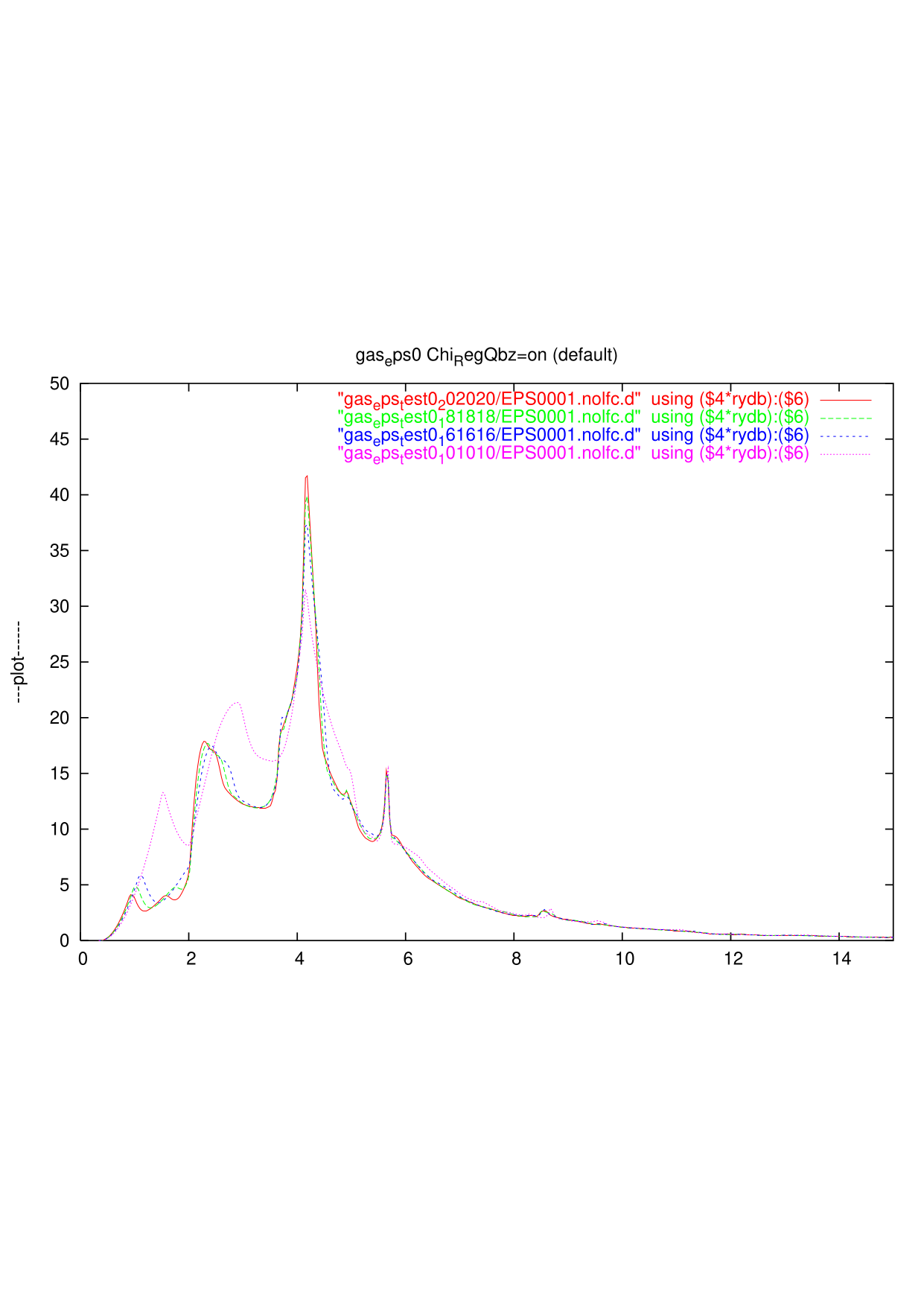 fig002: n1n2n3 convergence for Chi_RegQbz = off case. (mesh not including Gamma)
 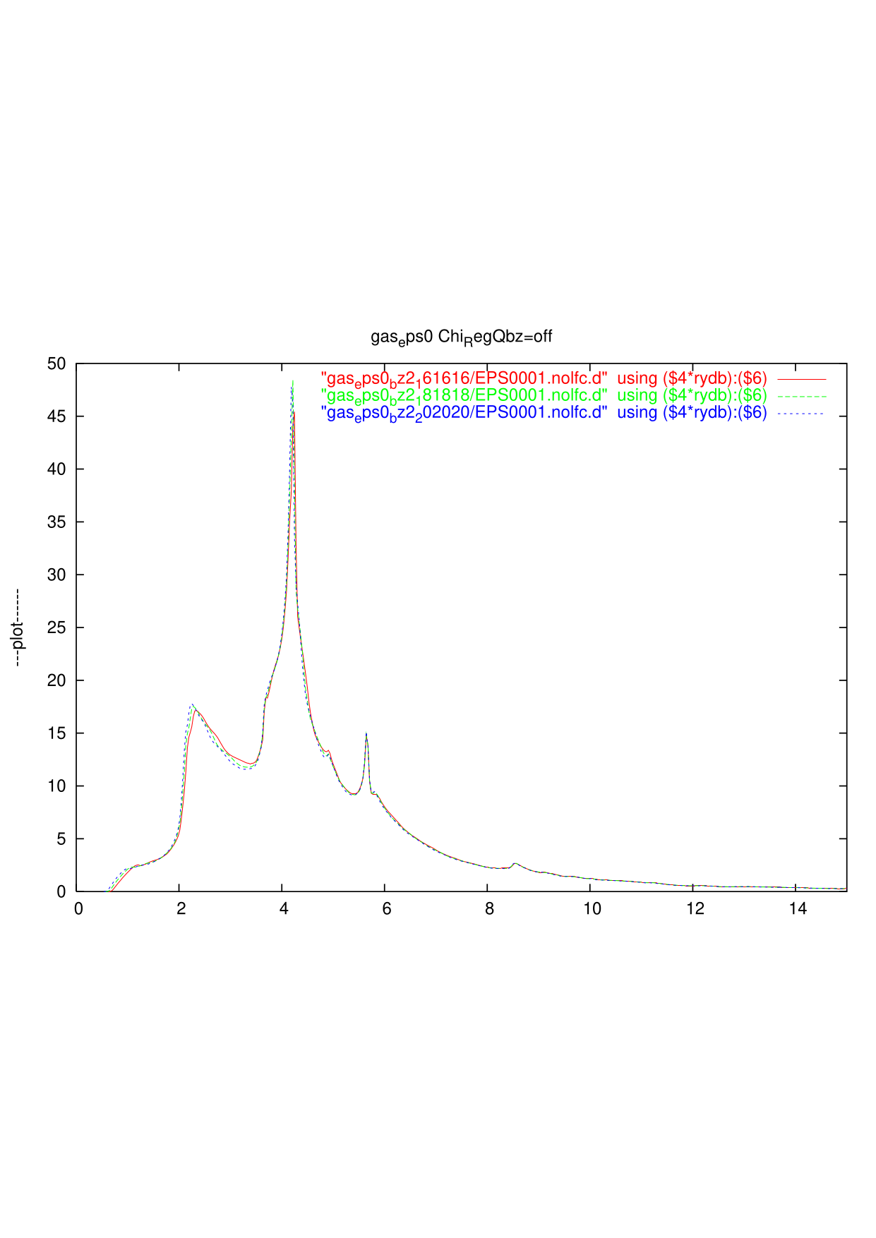 fig003: Alouanis'(from Arnaud) vs.
 Chi_RegQbz = on'' vs.Chi_RegQbz = off'' As you see, the threshold of the Red line (20x20x20 Chi_RegQbz=on) and Alouani's are almost the same, but the red line is too oscilating at the low energy part. On the other hand, ``Chi_RegQbz = off'' in Green broken line is not so satisfactory at the low energy part.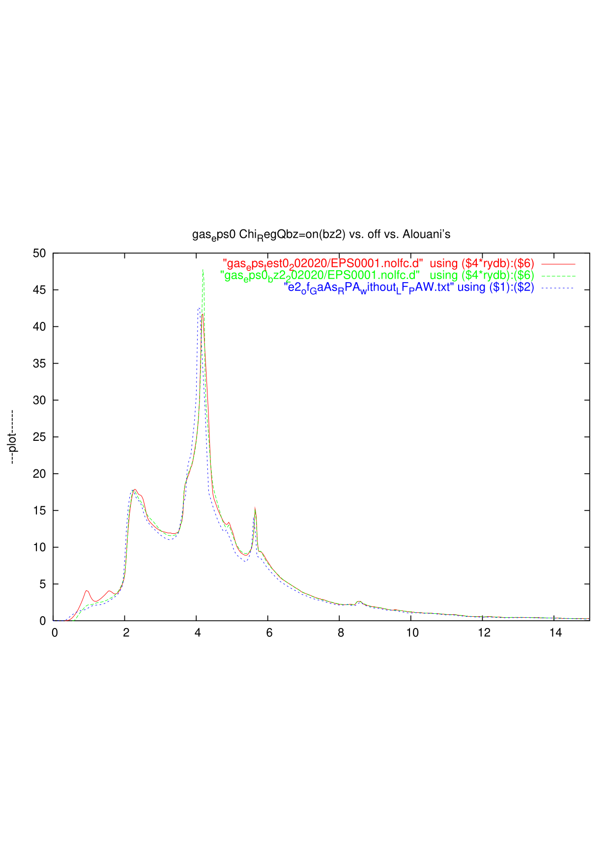
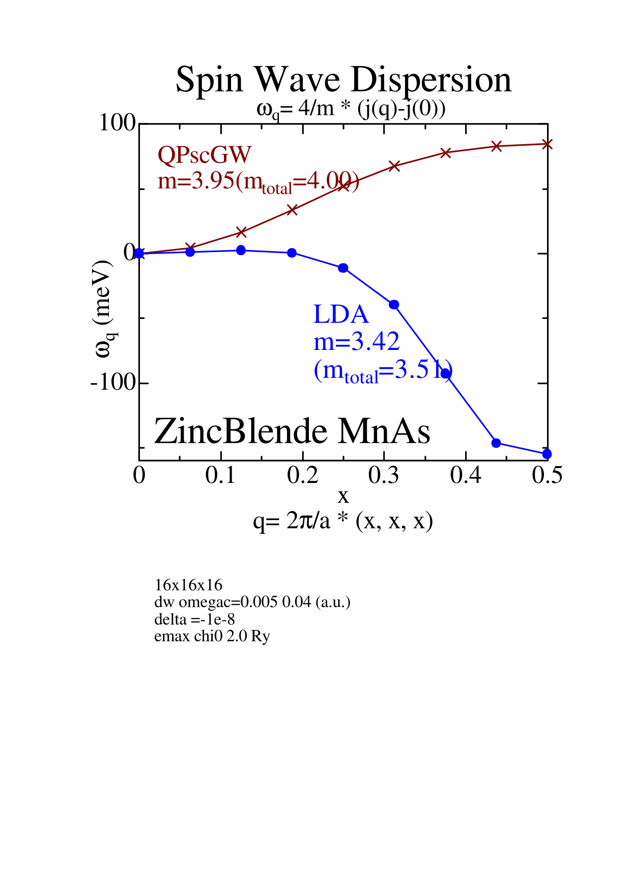
Old unpublished result for spin wave of ZB MnAs in QSGW as