UsageDetailed

console output

Console output is now mainly for debug purpose. But we still need to read some of output data from the console output (we are trying to modify this). From console output, we can check convergence behevior, band energies, Fermi energies, whether sigm, rst are correctly read in or not.

save.foobar

save.foobar records starting history invoking lmf,lmchk, and lmfa. In addition, it give total energies, a line per iteration of lmf. At each line,'i: intermediate, c: converged, x:iteration max without converged'.
In addition, -vfoobar=xxx is recorded (overriding variables in ctrl).
Two total energies Kohn-Sham and Harris-Folker is given---both should be virtually the same. But some differences for bigger systems. Take one of them.
log file log.foobar generated by lmf,lmchk,lmfa are currently used for debuggging purpose.

Spin polarized case without SOC

To treat magnetic systems, we have to set MMOM (ititial condition of spin magnetic moments) in addition to set nspin=2 in ctrl.foobar. The spin magnetic moments are specified as the difference of number of electrons between spin channels, isp=1 and isp=2.

For example, run

./job_materials.py NiO

at ecalj/MATERIALS/. For safe, it might be better to remover ecalj/MATERIALS/NiO/ in advance. Then we see console output ending with

...
Finished!: tail NiO/save.nio:c mmom= 0.0000 ehf(eV)=-86704.349038 ehk(eV)=-86704.348942 sev(eV)=-142.498970
============ end  ================================

. Try cat save.nio at ecalj/MATERIALS/NiO/. It shows iteration history of lmf. Last line in save.nio should show c mmom= 0.0000 ehf(eV)=-86704.349038 ehk(eV)=-86704.348942 sev(eV)=-142.498970 (energies may be slightly different). c means converged. ehf and ehk are total energies by two formulas. Note that total energy is not meaningful in QSGW

Look into ctrl.nio, which is generated from ctrls.nio supplied by the mini database handled by job_materials.py ctrl.nio contains

SITE    ATOM=Niup POS=  .0   .0   .0 # ← Niup site 
        ATOM=Nidn POS= 1.0  1.0  1.0 # ← Nidn site
        ATOM=O POS=  .5   .5   .5
        ATOM=O POS= 1.5  1.5  1.5
SPEC
    ATOM=Niup Z=28 R=2.12
      MMOM=0 0  1.2 0　       # ← initial spin
      EH=-1 -1 -1 -1  RSMH=1.06 1.06 1.06 1.06 
      EH2=-2 -2 -2  RSMH2=1.06 1.06 1.06 
      KMXA={kmxa}  LMX=3 LMXA=4 NMCORE=1
    ATOM=Nidn Z=28 R=2.12
      MMOM=0 0 -1.2 0        # ← initial spin
      EH=-1 -1 -1 -1  RSMH=1.06 1.06 1.06 1.06 
      EH2=-2 -2 -2  RSMH2=1.06 1.06 1.06 
      KMXA={kmxa}  LMX=3 LMXA=4 NMCORE=1

Here we have two sites named Niup and Nidn. MMOM=0 0 1.2 0 means initial spin moment within MTs: that is MMOM= {s} {p} {d} {f}, where {s} {p} {d} {f} are number of spin moments for each at atomic sites. Separators after MMOM can be space or comma. In addition, we set nspin=2 defined at the % const line in ctrl file.

Calculated spin moments within MT are at 'true mm' column in the console output, and shown in the mmom.nio.chk as

# Qtrue    MagMom(up-dn) Rmt   MT
1 8.527587  1.200085  2.120000 Niup    
2 8.527604 -1.200081  2.120000 Nidn    
3 5.380352 -0.000002  1.700000 O       
4 5.380352 -0.000002  1.700000 O

Note it is overwritten at every iteration. These are shown in concole output as `true mm' as well. Atomic site index are given in 'Siteinfo.chk'. Total Magnetic Moments are shown as

 Magnetic moment=     2.241805 !this is a case of bulk Fe

With the setting in GWinput generated by job_materials.py NiO, we can run gwsc as

gwsc -np 32 5 nio

I needed 275 sec with 32 MPI per QSGW cycle. I used this qsub script.

!/bin/sh
#$ -N NioTest
#$ -pe smp 32
#$ -cwd
#$ -M takaokotani@gmail.com
#$ -m be
#$ -V
#$ -S /usr/bin/bash
export OMP_NUM_THREADS=1
EXEPATH=/home/takao/bin/
$EXEPATH/gwsc -np 32 5 nio >& lgwsc

After calculations, remove temporary files with rm __* or cleargw ., which were already in your bindir. You can run job_band and so on in the same manner of DFT with nspin=1.

cat save.nio shows total energies (but not meaningufl)
We can effectively use antiferro symmetry for calculation (only for so=0,2)

orbital moments

When so=1, orbital moments within MTs are shown in at orbitalmom.chk: in the console output as

IORBTM:  orbital moments :
 ibas  Spec        spin   Moment decomposed by l ...
    1    Pr           1    0.000000   -0.011483   -0.010535   -4.881144    0.000234
    1    Pr           2    0.000000    0.012332    0.003604    0.000373   -0.000090
 total orbital moment   1:   -4.886708
    2    N            1    0.000000   -0.004174    0.001584    0.000291    0.000129
    2    N            2    0.000000    0.004622    0.000236    0.000045    0.000006
 total orbital moment   2:    0.002738

Antiferro symmetry without SOC

We can perform LDA/QSGW calculation with the AF symmetry (not for SOC=1). Only up spin are calculated. Then charge density and eigenvalues are symmetrized for the antiferro symmetry.

See ~/ecalj/Samples/AFsymmetry. To set AF symmetry, We have to set a line in ctrl file as

SYMGRPAF i:(1,1,1)  #Antiferro symmetry operation

Here SYMGRPAF is the generator of the antiferro magnetic symmetry that `g = i:(1,1,1) * should be the generator of magnetic space group, whereas

SITE    ATOM=Niup POS=  .0   .0   .0  AF=1    #Antiferro pair
        ATOM=Nidn POS= 1.0  1.0  1.0  AF=-1

should contains the AF= to specify antiferro pairs. Note that the space group operation i:(1,1,1) (this is inversion with translation) is explained at SYMGRP.

In addition, we have an example of ctrl.nise for NiSe.

  SYMGRPAF  i:(0,0,1/2)
  ATOM=Niup POS=     0.00       0.000   0.000 AF=1
  ATOM=Nidn POS=     0.00       0.000   0.500 AF=-1

, where inversion with (0,0,1/2) translation gives AF symmetry.

(README_mmtarget.aftest.txt shows the fixed-moment method for antiferro symmetry ---> need to be fixed).

Spin-orbit coupling

We have a switch HAM_SO in the ctrl file

For LDA/GGA, set nspin=2 and so=1. Then we can perform calculations including SOC. so=1 is for soc included (so=2 is for LzSz mode neglecting LxSz+LySy.
In the case of semiconductors such as GaAs, we need to include so=1 to see the band structure at the top of valence.
Currently, QSGW can not be performed with so=1. So we first have to run gwsc with so=0 or 2. After we get sigm file, we run lmf with --vso=1 (nit=1 can be fine) as a perturbation.
We can treat only colinear spins. Spin axis is along (0,0,1) as default. We can choose other direction with SOCAXIS. See ecalj/Samples/SOCAXIS. Not checked completely, but it seems work well.

Band plot with spin orbit coupling.

method 1: only apply SOC for band plot
bash
```
job_band mp-2534 -np 8 -vso=1 -vnspin=2
```
Caution: when you set nspin=2, the size of rst is twiced. No way to move it back to rst for nspin=1. So you may need to keep rst.
method 2. single iteration and SO=1
bash
```
mpirun -np 8 lmf -vso=1 -vnspin=2 -vnit=1
```
Then we have revised rst.foobar. Then run job_band mp-2534 -np 8 -vso=1 -vnspin=2.
method 3. full iteration SO=1
bash
```
mpirun -np 8 lmf -vso=1 -vnspin=2 -vnit=1
```
Then run job_band mp-2534 -np 8 -vso=1 -vnspin=2

Forces and Atomic position relaxiation

See ecalj/Samples/LaGaO3_relax. We have to set DYN category (only relaxiation). We can set directions for relaxation with SITE_ATOM_RELAX 0 0 1 or so. No cell optimizations.

CAUTION: For DYN mode, we treat the atomic position file AtomPos.lagao3. If it exists, we use atomic positions written in the file. See ecalj/SRC/subroutins/main_lmf.f90. You find call ReadAtomPos(irpos) which override positions specified by ctrl file. I have checked relaxation of the Perovskite LaGaO3 worked well. Since we do not use so much about the relaxation mode, be careful (I think some possible developments since atomic forces calculated well).

Fermi surface

See a sample at ecalj/Samples/FermiSurface Run job_fermisurface cu -np 4 10 10 10 after ctrl.cu converged. This write down all band energies (around Ef) for 10x10x10 in BZ. Then we can view it with xcrysden as xcrysden --bxsf fermiup.bxsf With –allband option to job_fermisurface, we have all the bands. Then we can see iso-energy surface at any energy.

PROCAR mode

See a sample at ecalj/Samples/MgO_PROCAR We can generate PROCAR file containing the size of eigenfuncitons**2. The sample (run job file) generates eps file showing fat band of O2 compon`ents. Run jobprocar. This gives *.eps file which shows Fat band picture. PROCAR (vasp format) is generated and analysed by a script BandWeight.py.

Spectrum of the Green's function

(under construction ...) spectrum of G

LDA+U

We have samples

https://github.com/tkotani/ecalj/tree/master/Samples/GdNldau
~/ecalj/Samples/ReNcub
IDU=, UH=, JH= specify parameters for LDA+U. IDU=#,#,#,... specifies which l-channels are to have U and the type of LDA+U implementation. 0 in a particular l-channel means no U is to be applied, 1 or 2 are for particular forms of LDA+U. For example, IDU= 0 0 0 1 UH= 0 0 0 -0.28 JH=0 0 0 0

BoltTrap

--boltztrap option is to generate files required for boltztrap. See ~/ecalj/Samples/Boltztrap

Dielectric function

~/ecalj/Samples/EPS Dielectric functions for Cu and GaAs. For Cu, we have intraband and interband contributions separately. See dielectric fuctnion.

Impact ionization rate

~/ecalj/Samples/IIR

Spin fluctuation

~/ecalj/Samples/Magnon It is via the MaxlocWannier. We are going to move to MLO instead. Here is a figure (this is on top of LDA) for the spin fluctuation of Fe in Okumura2021. 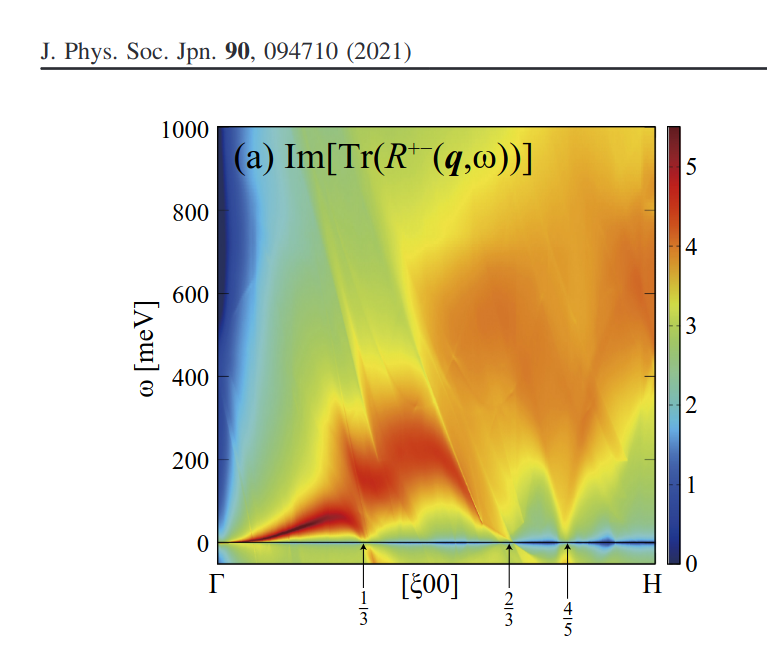alt text

Effective Screening Medium (ESM)

We can apply electric field to slab model. ESM combined with QSGW is quite unique. Used in the paper https://journals.aps.org/prb/abstract/10.1103/PhysRevB.101.205120 Ask us.

lmf and ctrl

See lmf and ctrl

gwsc and GWiput

See gwsc. For GPU, see ecaljgpu and gwsc for GPU for ISSP together. See explanation of GWinput.

getsyml: automatic symmetry line and BZ for band plot

See syml

These citations are required. 1.Y. Hinuma, G. Pizzi, Y. Kumagai, F. Oba, I. Tanaka, Band structure diagram paths based on crystallography, Comp. Mat. Sci. 128, 140 (2017) 2.Cite spglib that is essential for getsyml.

ecalj/Samples/

MLO: new localized basis Maximally localized Wannier function and cRPA interaction
MLWF_samples Wannier function generator and cRPA wannier90 method implemented in ecalj and cRPA. (a cRPA method by Juelich group). See Samples_MLWF/README. ~/ecalj/README_wannier.md This is going to be replaced with README_MLO.md
mass_fit_test Effective mass calculation. See README. probably not maitained\dots

ecalj_auto

This is a suit of python scripts to run thousands of gwsc calculations automatically. ecalj_auto

Background charge and fractional Z

backcround charge

How to perform paper-quarilty QSGW calculations with minimum costs.

The accuracy of band gaps can be ~0.1eV or larger for larger band gap materials.. In cases, it is easy, but in cases not so easy. So, it is better to use your own "simple criterion". "Not stick to convergence so much. Just stick to Reproducibility."

4f and 5f atoms

We need special care to tread atoms where 4f and 5f are fractionally filled. We have not yet include following setting in ctrlgenM1.py as for 4f/5f atoms (2025-08-07).

Here is the setting for RareEarth rocksalt nitrides ReN such as ErN.

Set nsp=2, so=2 (since QSGW can not treat so=1 now). (If necessary set so=1 after QSGW).
SYMGRP r4z. This is needed since we have lower symmetry rather than the lattice. It fixes the direction of spins and orbital moments.

Our setting is

--- ctrl.ern
  ATOM=Er Z=68 R=2.58
      PZ=0,5,0,5
      IDU=0 0 0 12  UH=0 0 0 0.773  JH=0 0 0 0.0945  MMOM=0 0 0 3
      EH=-1 -1 -1 -1  RSMH=1.29 1.29 1.29 1.29
      EH2=-2 -2 -2 -2  RSMH2=1.29 1.29 1.29 1.29
      KMXA={kmxa}  LMX=3 LMXA=6 NMCORE=1
      (pwemax=2, nk=8 8 8 was used)
--- GWinput
(n1n2n3 6 6 6 was used)
(tol 1d-2 was used)
lcutmx(atom)
6 2

Here PZ is the principle quantum number of local orbitals. This sets 5p and 5f as local orbitals. Run lmfa crn|grep conf to check atomic configulation.

IDU,UH,JH are the LDA+U parameters, only for initial condition. Since IDU is 10+2, we skip U effect when sigm exists.
MMOM is the initial magnetic moments.
LMXA=6 to expand augmented waves is needed.
Make sure READP=T.

With these settings, we can perform series of calculations finished for 4f ReN. Input files are available from here. Ask us when you like to use them.

QPU and QPD files

This contains the contents of self-energy

Papers

It is instractive to reproduce samples in Deguchi paper. We can set up templates for your calculations. Ask us. We have a latest paper at https://arxiv.org/abs/2506.03477 for GPU version. It shows some details of computational steps in ecalj. In Japanese, pages by Dr.Gomi at http://gomisai.blog75.fc2.com/blog-entry-675.html and https://qiita.com/takaokotani/items/9bdf5f1551000771dc48.

How to perform paper-quarilty QSGW calculations with minimum costs.

We expect that the accuracy of band gaps can be ~0.1eV (or larger for larger band gap materials). In cases, it is easy but in cases not so easy (magnetic metals requires many number of iterations). So, it is better to use your own "simple criterion". "Not stick to convergence so much. Just stick to Reproducibility."

LDA calculation

We need to confirm LDA-level of calculations first. The ctrl file is generated just from ctrls.* (crystal structure file) For calculation of QSGW, use large enough NKABC, so as to avoid convergence check on them.

QSGW: how to check convergence

QSGW iteration cycle by gwsc contains (1) and (2) (1) One-body self-consistent calculation (where we add sigm = Sigma-Vxc^LDA to one-body potential). to determine one-body Hamiltonian . (2) For given , we calculate sigm file.

Big iteration cycle of QSGW is made from (1)+(2). (gwsc script. not run_arg is a subroutine of bash script) With (1), we have small iteration cycle of one-body calculaiton with keeping given sigm.

In save.*, we see total energy (but not the total energy in the QSGW mode with sigm file), a line per each iteration of (1). A line "c ..." is the final iteration cycle of (1)."x ..." is unconverged (but no problem as long as we finally see "c ...").

The command "grep '[cx] ' save.*" gives an indicator for going to be converged or not. Or you can take "grep gap llmf.*run" (see it bottom.)

Another way: dqpu QPU.3run QPU.6run is to compare two QPU files which contains QP energies. (note: QP energies shown are calculated just at the begininig of iteration).

For insulators, (I think), comparing band gap for each iteration is good enough to check onvergence. But for metal, it is better to plot energy bands for some of final iterations, and overlapped(cd QSGW.*run and run job_band).

Another way is grep rms lqpe*. This gives rmsdel. Diffence of self-energy (at least we see it is getting smaller for initial first cycles).

How to make 80%QSGW +20% LDA, and SO setting

Note that sigm file contains . If sigm exists, lmf read it, and run self-consistent calculations with adding sigm to the one-body potential.

Justifications of QSGW80 are:

1. QSGW80(NoSC)

For practical prediction of band structure, such as band gap and so on, it may be better to use 80% QSGW +20% LDA procedure when you make band plot. After, you have rst and sigm files determined self-consistently Run

job_band gaas -np 4 -vssig=0.80

(Confirm ssig is defined and cited as ScaledSigma={ssig} in the ctrl file). This gives a result of QSGW80nosc in the TableII.

2. QSGW80(Nosc)+SO

80%QSGW+20%LDA with SO=1 (L.S method). If you like to include L.S method

mpirun lmf gaas -np 4 -vssig=0.80 -vso=1 -vnspin=2

This procedure makes self-consistency with keeping the sigm file. This may/(or may not) required. If you expect large obital moment this procedure may be needed.

job_band gaas -np 4 -vssig=0.80 -vso=1 -vnspin=2

NOTE: nspin=2 is required for so=1. rst and sigm are expanded for npsin=2 (you can not run with nspin=1, after rst and sigm are expanded).

3. QSGW80

With ssig=0.80, you can run QSGW calculaiton in gwsc. Then you have self-consistent results of QSGW80. You can simultaneously use the setting so=2 (Lz.Sz scheme). Be careful for z-direction and setting of SYMOPS (so as to keep the z-axis), for so=2. If you like to get results of QSGW80+SO, you need to set so=1 after self-consistent of sigm atteined.

4. Example of GaAs

Good example to check band gap, and SO splitting at top of valence of Gamma point for ZB structure as GaAs. Before run it, make sure your ctrl file include variables ssig, so, nspin by

>grep ssig ctrl.gaas
>grep so   ctrl.gaas
>grep nspin ctrl.gaas

to know the variable ssigm is defined and used as ScaledSigma={ssig}, NSPIN={nspin}. For -vso=1 work, you also need to so is defined and SO={so} is set in ctrl.

How to do version up? git minimum

Be careful to do version up ecalj. It may cause another problem. If you are not good at git, make another clone. Do not mix up with previous version (e.g. where you install)

cd ecalj
git log
This shows what version you use now.

git diff > gitdiff_backup This is to save your changes added to the original (to a file git_diff_backup ) for safe. I recommend you do take git diff >foobar as backup. git stash also move your changes to stash.

git checkout -f CAUTION!!!: this delete your changes in ecalj/. This recover files controlled by git to the original which was just downloaded.

git pull This takes all new changes. It is safer to use git fetch and gitk --all (git checkout FETCH_HEAD -b youbranch) to checkout your local branch.

I think it is recommended to use

gitk --all

and read this document. Difference can be easily taken, e.g. by

git diff d2281:README 81d27:README (here d2281 and 81d27 are several digits of the begining of its version id).

git show 81d27:README

is also useful.

error messages and caution

Bandplot for FSMOMMETHOD/=0

Even when you use FSMMOMMETHOD/=0 in GWinput for gwsc, you need to set FSMOMMETHOD=0 (or comment it out) when you run job_band_nspin2. [If you run job_band_nspin2 with FSMOMMETHOD/=0, it make a shift (adding bias magnetic field).] Anyway confusing. If necessary, I have to make it straight.

For molecules, we may use --systype=molecule for ctrlgemM1.py.

Then we have

TETRA=0 N=-1 #Negative is the Fermi distribution function W= gives temperature. W=0.001 #W=0.001 corresponds to T=157K as shown in console In addiiton, FSMOM (n_up-n_down) is needed (FSMOMMETHOD=1)if we have magnetic moment.

core>evalence message.

Ecore is grater than Evalence. For safe, we do not allow this. Compare ECORE file and valence levels, shown in log file or console output.

Back ground charge and fractional Z.

You can use fractional numbers for ATOM_Z, and also can set valence charge by BZ_ZBAK (I removed BZ_VAL). You see console out put, e.g,

Charges: valence 19.80000 cores 8.00000 nucleii -28.00000 hom background .20000 deviation from neutrality: 0.00000 This is a case with BZ_ZBAK=.2

NOTE: at the first iteration, Charges: shows such as

Charges: valence 8.00000 cores 20.00000 nucleii -28.00000 hom background 0.12300 deviation from neutrality: 0.12300

because of the initial condition by superposition of atoms. It shows deviation seems nonzero. But charge should be conserved from the next iteration.

convergence problem.

We need to use smaller ITER b, such as 0.015, 0.01, 0.005.

Use PZ or not.

If spillout of core is not so small (more then 0.05 or something.), it is better to use PZ(lo). Treat the core as valecne. Bi4d is such a case. Maybe use PZ=0,0,4.9

We use only CORE1 treatment only (exchange only core)

See 10.1103/PhysRevB.76.165106 (Eq.35 and after). Now I usually not use CORE2 (CORE1 only).

a little unstable when metal GGA, especially when we have large empty regions. (still problematic?)

(negative density points appears: console output). I am not so sure about this is serious or not.

total enegry is not meaningful in QSGW mode

Even gwsc, we see total energy in lmf cycle. But it might be taken just an indicator to the convergence.

Do we use VWN or GGA for QSGW? ===

In principle, QSGW results should not depend on VWN or GGA. But there is minor dependence, because

frozen core density.
core eigenfunctions.
radial basis functions
Slight numerical reason (This is probably because Sigma-interpolation procedure But not exactly figured out yet → affect about 0.02eV as for band gap for GaAs.). In anyway, use VWN (HAM_XCFUN=1) as standard. And such technical things affects, 0.05 eV level of error for band gap.

numerical accuaray of QSGW band energies

As for the band gaps 0.1 eV is a kind of limiting accuaray for usual semiconductors with 0~3 eV band gap materials. For Si or something simple, you may be able to have better accuracy. However, QSGW is on the so many parameters. So, just say ~0.1eV level of accuracy. Convergence check is expected for the technical developments in future.

TOTE files

In gw_lmfh, hqpe gives TOTE.UP and QPU files (DN and QPD as well). They contains the same values.

The Fermi energies in GW

We use two kinds of Fermi energy and . This is because of numerical techniques.

One is , contained in EFERMI, for the polarization function since we use tetrahedron method for it.

The other is for $ G \times W$ since we use smeared pole technique for . is given at the beginning of $ G \times W$ calculations. See lsx,lsc,lsxC (for mpirun, we have them in stdout.0000*).

Anisotropic Q0P

In cases, we are worrying about the anisotropy. The offset Gamma method uses the 1/10 of gamma cell. It seems not so bad, however, we may need to examine the anisotropy problem again in future.
It is problematic to use unbalanced k points for anisotropic cell. See Copmuter Physics Comm. 176(2007)1-13.

mixbeta and mixpriorit

If not stable convergence in gwsc, try to set mixbeta 0.5 in GWinput.

Check Used MTOs

Near beginig of console output, what MTO you use is shown as: (GaAs case).

sugcut:  make orbital-dependent reciprocal vector cutoffs for tol= 1.00E-06
spec      l    rsm    eh     gmax    last term    cutoff
 Ga       0*   1.13  -1.00   6.579    1.19E-06    1459
 Ga       1*   1.13  -1.00   7.028    1.26E-06    1807
 Ga       2*   1.13  -1.00   7.475    1.09E-06    2109
 Ga       3    1.13  -1.00   7.920    1.06E-06    2637
 Ga       0*   1.13  -2.00   6.579    1.19E-06    1459
 Ga       1*   1.13  -2.00   7.028    1.26E-06    1807
 Ga       2    1.13  -2.00   7.475    1.09E-06    2109
 As       0*   1.18  -1.00   6.300    2.13E-06    1243
 As       1*   1.18  -1.00   6.720    1.26E-06    1471
 As       2*   1.18  -1.00   7.140    1.37E-06    1837
 As       3    1.18  -1.00   7.558    1.05E-06    2229
 As       0*   1.18  -2.00   6.300    2.13E-06    1243
 As       1*   1.18  -2.00   6.720    1.26E-06    1471
 As       2    1.18  -2.00   7.140    1.37E-06    1837

one-show QSGW (not one-shot GW)

one-shot QSGW can be useful in cases. As it contains off-diagonal part, we can resolve band tanglement problem in Ge (no band gap). one-shot GW is also used to calculate impact ionization rate.

Maxloc wannier. Maximally localized Wannier with effective interaction in CRPA.

Our own implementation of Wannier90 is included. It works with the command genMLWF, where we can run cRPA in it.

We can generate Wannier functions in the manner of Wannier90 by the script genMLWF. It automatically performs cRPA calculation (formulation given by Juelich group) successively. genMLWF is the script to generate the Wanneir functions. In addition, it gives effective interaction in CRPA.

Required setting is written in the GWinput. We have examples in ecalj/Samples/MLWF_samples which contains CuMLWFs, Cu, Fe, NiOMLWF, SrVO3 but some may be missing.

Run a sample at Samples/MLWF_samples/CuMLWFs

See ./job file. Run this or run one by one as follows. At firts, run self-consistent calculation as

lmfa cu
mpirun -np 8 lmf cu
job_band cu -np 8

(it is possible to start from QSGW results). Then we run main script of maxloc wannier with effective interaction W as

genMLWF -np 8 cu

The setting needed for the Wannir is 1. Orbital setting and window settings. These are
```
<Worb> Site
1 Cu 5 6 7 8 9
</Worb>
wan_out_emin -10  !eV relative to Efermi
wan_out_emax -1   !eV relative to Efermi
```
for Cu 3d. For the sample of NiO, we set
```
<Worb> Site
1 Niup   5 6 7 8 9
2 Nidn   5 6 7 8 9
!  3 O   1 2 3 4 5 6 7 8 9 10 11 12 13 14 15 16
!  4 O   1 2 3 4 5 6 7 8 9 10 11 12 13 14 15 16
</Worb>
wan_out_emin -4    !eV relative to Efermi
wan_out_emax  2    !eV relative to Efermi
```
Here we specify seed funcitons for which we have Wannier functions. This specify we tread bands for Ni. We can set inner window as well if we set
```
wan_in_ewin on
wan_in_emin  -4  !eV relative to Efermi
wan_in_emax   0  !eV relative to Efermi
```
- Wannier is generated at echo 2|hmaxloc >lmaxloc2 (look into genMLWF). At this point, you can make band plot to check whether your setting for Wannier work well or not; the model-Hilbert space by band plot. (we need syml.* file and run job_band to get original energy bands) Then plot wannier band on top of it. See Samples/MLWF_samples/CuMLWFs/bandplot.MLWF.isp1.glt as an example. If the plot is strange, you need to choose outer and inner windows for Wannier.
  (Repeat echo 2| hmaxloc >lmaxloc2 until you have satisfactry fitting with changing the setting wannier part in GWinput ).

output

*** Band plot including Wannier band See bandplot.MLWF.isp1.glt

Look into CuMLWFs/bandplot.MLWF.cu.glt This is for interpolated band. A line "bnds.maxloc.up" u ($5):($6+de) lt 3 w l ti "Wannier" is added to usual output of bandplot.cu.isp* given by job_band.
** NOTE: Efermi shift: genMLWF requies bnds.${target} to read the Fermi energy. To generate it, we need to run job_band in advance. Or run,
```
echo 2 | hmaxloc  > lmaxloc2
```
(need syml*); this can be runned after genMLWF. (Or need to shift Ef by hand as follows in gnuplot script.)
```
de = ((ef shown in "lmaxloc2") - (ef in llmf_ef(bnds.${target}))*13.605
plot \
"bnd1.dat" u 2:3 lt 1 pt 1 not w l,\
"bnd2.dat" u 2:3 lt 1 pt 1 not w l,\
"bnd3.dat" u 2:3 lt 1 pt 1 not w l,\
"bnd4.dat" u 2:3 lt 1 pt 1 not w l,\
"bnd5.dat" u 2:3 lt 1 pt 1 not w l,\
"bnds.maxloc.up" u ($5):($6+de) lt 3 w l ti "Wannier"
```

xxx(2) Plot psi.xsf file. xxx xxx Not working xxx I currently surpress wanplot, which plots MaxLoc Wannier functions in real space xxx So vis_* options for plot in GWinput is not working. xxx (Skipped now) Wannier funciton plot xxx Use wan.xsf by Xcrysden (skipped now) xxx Range of plot looks not good; xxx Especially, vis_wan_ubound, vis_wan_lbound should be not integer. xxx Probably, need to improve/(bug fix) wanplot.F.

We get three files (see genMLWF) containing v and W-v information. grep "Wannier" lwmatK1 > Coulomb_v grep "Wannier" lwmatK2 > Screening_W-v grep "Wannier" lwmatK3 > Screening_W-v_crpa These are text files <ab|W|cd> element. a,b,c,d are index of Wannier functions (ask us if necessary). Then we have Static_W.dat (RPA) and Static_U.dat (cRPA). These contains static U, U', J, and J' (\omega = 0). For example,
```
grep '    1    1    1    1    1'             Coulmb_v
grep '    1    1    1    1    1    0.000000' Screening_W-v.UP
grep '    1    1    1    1    1    0.000000' Screening_W-v.crpa
```
shows
```
Coulomb_v.UP:          Wannier ...  23.499183   -0.000000
Screening_W-v.UP:      Wannier ... -20.317956   -0.000000
Screening_W-v_crpa.UP: Wannier ... -20.188076   -0.000000
```
This means
```
<11|W|11>     =23.499183-20.317956
<11|U_CRPA|11>=23.499183-20.188076
```
Note that this is by the test example CuMLWFs, not so reliable numerically.

With the command grep Wan lwmatK*, we can see (This case : Cu cases). Then compare these with Result.grepWanlwmatK These are onsite effective interactions (diagonal part only shown).

lwmatK1:  Wannier    1    1   24.644475    0.000000 eV
lwmatK1:  Wannier    1    2   24.644576    0.000000 eV
lwmatK1:  Wannier    1    3   25.471361    0.000000 eV
lwmatK1:  Wannier    1    4   24.644575    0.000000 eV
lwmatK1:  Wannier    1    5   25.470946    0.000000 eV
lwmatK2:  Wannier    1    1    0.000000 eV   -21.263759   -0.000000 eV
lwmatK2:  Wannier    1    2    0.000000 eV   -21.263839    0.000000 eV
lwmatK2:  Wannier    1    3    0.000000 eV   -21.931033   -0.000000 eV
lwmatK2:  Wannier    1    4    0.000000 eV   -21.263839   -0.000000 eV
lwmatK2:  Wannier    1    5    0.000000 eV   -21.930702   -0.000000 eV

These are the diagonal elements , where corresponding to the orbitals (real harmonics).

Some additional info in README_wannier.md Time consuming part (and also the advantage) is for effective interaction in RPA. Look into the shell script genMLWF; you can skip last part if you don't need the effective interaction.

History (not latest description)

alt text

UsageDetailed ​

console output ​

save.foobar ​

Spin polarized case without SOC ​

orbital moments ​

Antiferro symmetry without SOC ​

Spin-orbit coupling ​

Band plot with spin orbit coupling. ​

Forces and Atomic position relaxiation ​

Fermi surface ​

PROCAR mode ​

Spectrum of the Green's function ​

LDA+U ​

BoltTrap ​

Dielectric function ​

Impact ionization rate ​

Spin fluctuation ​

Effective Screening Medium (ESM) ​

lmf and ctrl ​

gwsc and GWiput ​

getsyml: automatic symmetry line and BZ for band plot ​

ecalj/Samples/ ​

ecalj_auto ​

Background charge and fractional Z ​

How to perform paper-quarilty QSGW calculations with minimum costs. ​

4f and 5f atoms ​

QPU and QPD files ​

Papers ​

How to perform paper-quarilty QSGW calculations with minimum costs. ​

LDA calculation ​

QSGW: how to check convergence ​

How to make 80%QSGW +20% LDA, and SO setting ​

1. QSGW80(NoSC) ​

2. QSGW80(Nosc)+SO ​

3. QSGW80 ​

4. Example of GaAs ​

How to do version up? git minimum ​

error messages and caution ​

Bandplot for FSMOMMETHOD/=0 ​

For molecules, we may use --systype=molecule for ctrlgemM1.py. ​

core>evalence message. ​

Back ground charge and fractional Z. ​

convergence problem. ​

Use PZ or not. ​

We use only CORE1 treatment only (exchange only core) ​

a little unstable when metal GGA, especially when we have large empty regions. (still problematic?) ​

total enegry is not meaningful in QSGW mode ​

Do we use VWN or GGA for QSGW? === ​

numerical accuaray of QSGW band energies ​

TOTE files ​

The Fermi energies in GW ​

Anisotropic Q0P ​

mixbeta and mixpriorit ​

Check Used MTOs ​

one-show QSGW (not one-shot GW) ​

Maxloc wannier. Maximally localized Wannier with effective interaction in CRPA. ​

Run a sample at Samples/MLWF_samples/CuMLWFs ​

output ​

History (not latest description) ​

UsageDetailed

console output

save.foobar

Spin polarized case without SOC

orbital moments

Antiferro symmetry without SOC

Spin-orbit coupling

Band plot with spin orbit coupling.

Forces and Atomic position relaxiation

Fermi surface

PROCAR mode

Spectrum of the Green's function

LDA+U

BoltTrap

Dielectric function

Impact ionization rate

Spin fluctuation

Effective Screening Medium (ESM)

lmf and ctrl

gwsc and GWiput

getsyml: automatic symmetry line and BZ for band plot

ecalj/Samples/

ecalj_auto

Background charge and fractional Z

How to perform paper-quarilty QSGW calculations with minimum costs.

4f and 5f atoms

QPU and QPD files

Papers

How to perform paper-quarilty QSGW calculations with minimum costs.

LDA calculation

QSGW: how to check convergence

How to make 80%QSGW +20% LDA, and SO setting

1. QSGW80(NoSC)

2. QSGW80(Nosc)+SO

3. QSGW80

4. Example of GaAs

How to do version up? git minimum

error messages and caution

Bandplot for FSMOMMETHOD/=0

For molecules, we may use --systype=molecule for ctrlgemM1.py.

core>evalence message.

Back ground charge and fractional Z.

convergence problem.

Use PZ or not.

We use only CORE1 treatment only (exchange only core)

a little unstable when metal GGA, especially when we have large empty regions. (still problematic?)

total enegry is not meaningful in QSGW mode

Do we use VWN or GGA for QSGW? ===

numerical accuaray of QSGW band energies

TOTE files

The Fermi energies in GW

Anisotropic Q0P

mixbeta and mixpriorit

Check Used MTOs

one-show QSGW (not one-shot GW)

Maxloc wannier. Maximally localized Wannier with effective interaction in CRPA.

Run a sample at Samples/MLWF_samples/CuMLWFs

output

History (not latest description)