ecalj MainDocument

This is MainDocument of ecaljdoc. All files are linked from this file.

Here we give GetStarted, together with install and overview of QSGW.
We have UsageDetails in another file.
Qiita Japanese may be a help, but most of all are shown here.
When link did not work, go to https://github.com/tkotani/ecalj to download.

Licence

AGPLv3. For publications, we hope to make a citation as; [1] ecalj package available from https://github.com/tkotani/ecalj/.

Install

To install ecalj, look into install, as well as install for ISSP

Features of ecalj package

All electron full-potential PMT method The PMT method means; a mixed basis method of two kinds of augmented waves, that is, APW+MTO. In other words, the PMT method= the linearized (APW+MTO) method, which is unique except the Questaal having the same origin with ecalj. We found that MTOs and APWs are very comlementary, corresponding to the localized and the extented natures of eigenfunctions. That is, very localized MTOs (damping factor where $\kappa \sim 1 $ bohr; this implies only reaching to nearest atoms) together with APWs (cutoff is Ry) works well to get reasonable convergences. We can perform atomic-position relaxation at GGA/LDA level. Because of including APWs, we can describe the scattering states very well. 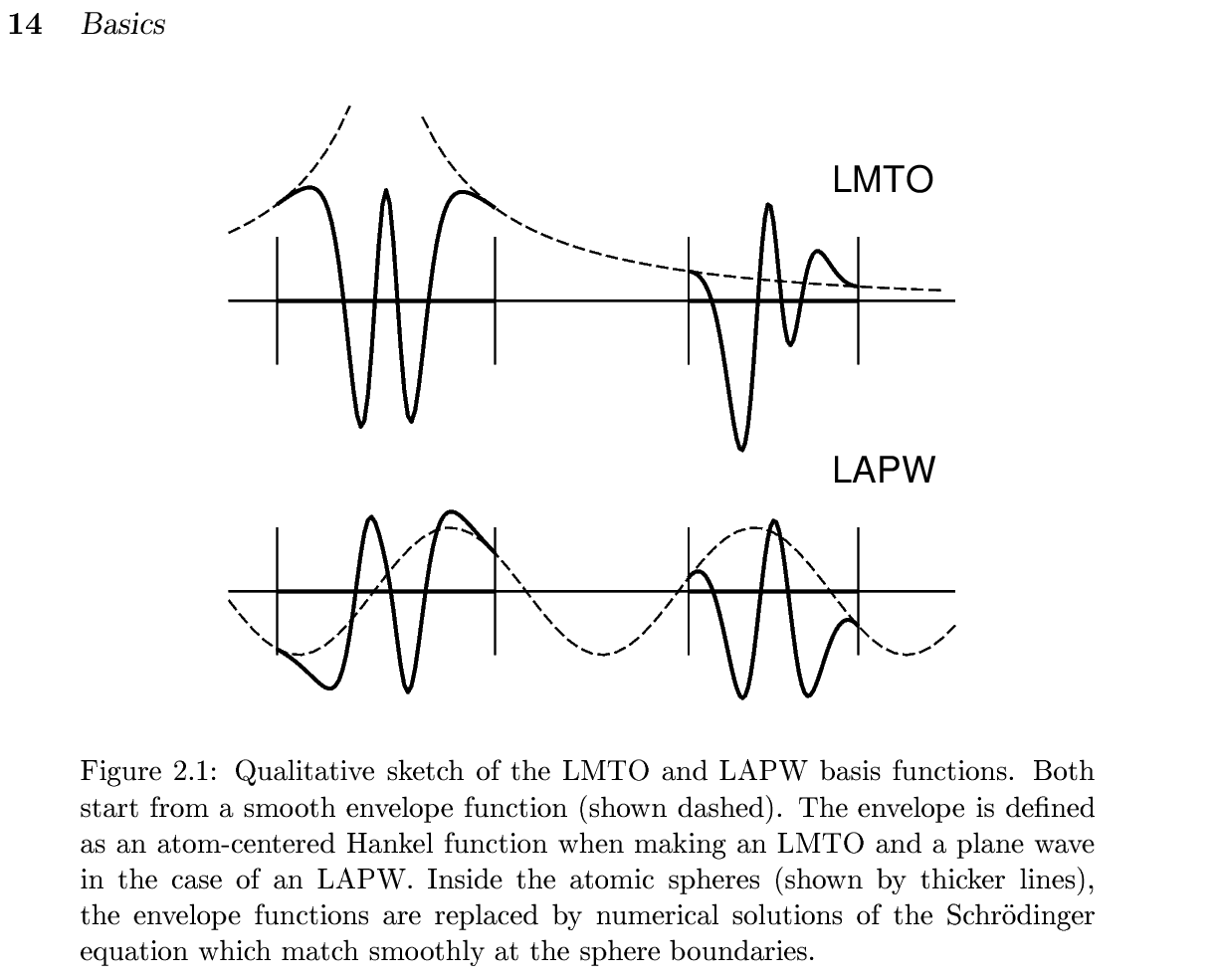(This fig is taken from nfp-manual by M. Methfessel and M. van Schilfgaarde) Our current PMT formulation is given in
[1]KotaniKinoAkai2015, PMT formalism
[2]KotaniKino2013, PMT applied to diatomic molecules.
Since we have automatic settings for basis-set parameters, we don't need to be bothered with the parameter settings. Just crystal structures (POSCAR) are needed for calculations.
- Original PMT was started at https://journals.aps.org/prb/abstract/10.1103/PhysRevB.81.125117
- PMT uses smooth Hankel functions described in the smooth Hankel paper by E. Bott, M. Methfessel, W. Krabs, and P. C. Schmidt, which was used in [B]nfp paper by M. Methfessel and M. van Schilfgaarde, and R.A. Casali. Our PMT is on top them.
- In addition to PMT basis, we use local orbitals together.
- The cutoff Ry may sound surprisingly small. However, note that high energy part of the plane wave methods are consumed only for the core like shape of eigenfunctions with negative curvatures of radial functions. Furthermore, the plane waves have difficulties not satisfying the periodic gauge https://arxiv.org/pdf/2010.03959. On the other hand, localized basis methods such as LMTO and Gaussians have difficulties to handle vacuum regions.
PMT-QSGW method
The PMT-QSGW means the Quasiparticle self-consistent GW method (QSGW) based on the PMT method. The development of [3] is the key to perform QSGW on the PMT. We can handle even magnetic metals. Since we have implemented ecalj on GPU, we can handle ~40 atoms with four GPUs. [3]Kotani2014, Formulation of PMT-QSGW method [4]D.Deguchi PMT-QSGW applied to a variety of insulators/semiconductors [5]M.Obata GPU implementation, where we treat Type II GaSb/InAs (40 atoms) with four GPUs. We can easily make band plots without the Wanneir kinds of interpolations. This is because an interpolation scheme of self-energy is internally built in. This is very essential to calculate physical quantities from eigenfunctions on top of the QSGW ground states.
Since we treat all the electrons, we are not bothered with the ambiguities of the pseudopotentials.
Dielectric functions and magnetic susceptibilities We can calculate GW-related quantities such as dielectric functions, spectrum function of the Green's functions, Magnetic fluctuation, and so on. Since our QSGW can generate eigenfunctions and eigenvalues at any k points.
The Model Hamiltonian with Wannier functions We can generate the effective model (Maxloc Wannier and effective interaction between Wannier funcitons). This is originally from codes by Dr.Miyake, Dr.Sakuma, and Dr.Kino. The cRPA given by Juelich group is implemented. Here is a latest paper to using this, https://journals.aps.org/prb/abstract/10.1103/PhysRevB.108.035141.
- We are now replacing MLWF with MLO (MuffinTinOrbail-based Localized Orbitals), where we can easily throw away (downfolding) the APW degree of freedom.
Singleton pattern in fortran The main part of our codes is in fortran. Our codes have the object-oriented structures respecting the singlton design pattern. We think this is a step to replace our fortran codes with those in modern languages such as JAX/PyTorch. Inevitably, we still have legacy codes but encapsulated as possible, and going to be replaced.

Overview of QSGW

Band calculations (LDA level) are performed with the program lmf. The initial setting file is ctrl.foobar ( foobar is user-defined). Before running lmf, it is necessary to run lmfa, which is a spherically symmetric atom calculation to determine the initial conditions for the electron density (lmfa finishes instantaneously).
A file sigm.foobar is the key for QSGW calculations. The file sigm.foobar contains the non-local potential . By adding this potential term to the usual LDA calculation performed by lmf, we can perform QSGW calculations. See figure below.
Thus the problem is how to generate . This is calculated from the self-energy , which is calculated in the GW approximation. Roughly speaking, we obtain with removing the omega-dependence in .
Therefore, the calculation of is the major part of the QSGW cycle, and is calculated in a double-structure loop. That is, there is an inner loop of lmf, and an outer loop to calculates using the eigenfunctions given by lmf. This outer loop can be executed with a python script called gwsc (which runs fortran programs). The computational time for QSGW is much longer than that of LDA calculation. As a rule of thumb, it takes about 10 hours for 20 atoms (depending on the number of electrons. For systems more than 10 atoms per cell or so, we recommend to use GPUs).
Here is the QSGW cycle shown in Figure 1 in https://arxiv.org/abs/2506.03477 . MPB meand the mixed product basis to expand products of eigenfunctions.
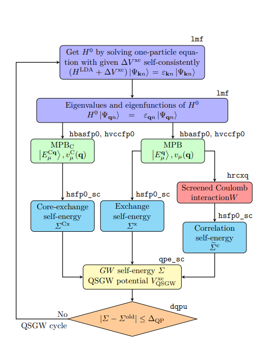
We have GPU acceleration for QSGW, which also describe basics of QSGW. QSGW algorism fits to GPU computations very well. With four GPUs, we can compute systems with 40 atoms per cell. (As for lmf part, GPUs are not efficiently used yet.). Our PMT allows us to handle large vaccum region for slab model.
We can perform QSGW virtually without parameter settings by hands. Thus I think ecalj is one of the easiest to perform GW/QSGW. See band database in QSGW at https://github.com/tkotani/DOSnpSupplement/blob/main/bandpng.md (this is a supplement of https://arxiv.org/abs/2507.19189). This is away from complete database, but showing the ability of ecalj.

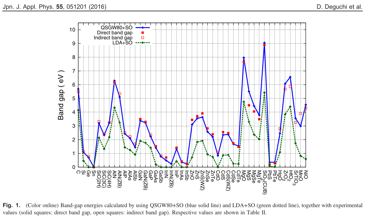alt text This is taken from [4]D.Deguchi

In comparison with LDA, we see differences in QSGW;

Band gap. QSGW tends to give slightly larger than experiments. It looks systematic as in the Figure above.
Band width. Usually, sp bands are enlarged (except very low density case such as Na). This is consistent with the case for homogeneous electron gas. Localized bands like 3d electrons get narrowed.
Relative position of bands. e.g. O(2p) v.s. Ni(3d). More localized bands tends to get more deeper. Exchange splitting between up and down get larger (like LDA+U) . In cases such as NiO, magnetic moment become larger; closer to experimental values.
Hybridization of 3d bands with others. QSGW tends to make eigenfunctions localized.

However, reality is complexed, and not so simple in cases.

GetStarted

Here we explain DFT/QSGW calculations with ecalj. Then we explain how to make band plots. For simplicity, we treat paramagetic cases (nsp=1), no 4f, no SOC. We explain things step by step.

Further details are explained at UsageDetailed

Step 0. Get POSCAR

We first need POSCAR (crystal structure in VASP format). You can find samples of POSCAR in ecalj/ecalj_auto/INPUT/testSGA/POSCARALL as

bash

cd ecalj
mkdir TEST
cd TEST
mkdir test1
mkdir test2
cat ecalj_auto/INPUT/testSGA/joblist.bk
cp ../ecalj_auto/INPUT/testSGA/POSCARALL/POSCAR.mp-2534 test1
cp ../ecalj_auto/INPUT/testSGA/POSCARALL/POSCAR.mp-8062 test2

For example, POSCAR of mp-2534 GaAs is given as:

Ga1 As1
1.0
   3.5212530000000002    0.0000000000000000    2.0329969999999999
   1.1737510000000000    3.3198690000000002    2.0329969999999999
   0.0000000000000000    0.0000000000000000    4.0659929999999997
Ga As
1 1
direct
   0.0000000000000000    0.0000000000000000    0.0000000000000000 Ga
   0.2500000000000000    0.2500000000000000    0.2500000000000000 As

This is POSCAR for ba2pdo2cl2 (QSGW results are shown below):

POSCAR_ba2pdo2cl2
1.0
-2.06443 2.06443 8.40383 
2.06443 -2.06443 8.40383 
2.06443 2.06443 -8.40383 
Ba Pd O Cl 
2 1 2 2 
Cartesian
0.0 0.0 6.5153213224
0.0 0.0 10.2923386776
0.0 0.0 0.0
0.0 2.06443 0.0
2.06443 0.0 0.0
0.0 0.0 3.1625293056
0.0 0.0 13.6451306944

If you have cif and like to convert it to POSCAR, do cif2cell foobar.cif -p vasp --vasp-cartesian --vasp-format=5.

Step 1. convert POSCAR to ctrls

Then we convert POSCAR to ctrls by vasp2ctrl. ctrls is the structure file used in ecalj.

vasp2ctrl POSCAR.mp-2534 
mv ctrls.POSCAR.mp-2534.vasp2ctrl ctrls.POSCAR.mp-2534
cat ctrls.mp-2534

ctrls.mp-2534 contains crystal structure equivalent to POSCAR:

STRUC
     ALAT=1.8897268777743552
     PLAT=       3.52125300000       0.00000000000       2.03299700000  
                 1.17375100000       3.31986900000       2.03299700000 
                 0.00000000000       0.00000000000       4.06599300000 
SITE
     ATOM=Ga POS=     0.00000000000       0.00000000000       0.00000000000 
     ATOM=As POS=     1.17375100000       0.82996725000       2.03299675000

Indentation is needed to show blocks of categories, STRUC and SITE. Another example of ctrls.GaAs

%const bohr=0.529177 a=5.65325/bohr
STRUC
     ALAT={a}
     PLAT=0 0.5 0.5 0.5 0 0.5 0.5 0.5 0
SITE
    ATOM=Ga POS=0.0 0.0 0.0
    ATOM=As POS=0.25 0.25 0.25

ctrls.srtio3:

%const au=0.529177
%const d0= a0=2*1.95/au v=a0^3 a1=v^(1/3)
STRUC ALAT={a1}
   PLAT=1 0 0 0 1 0 0 0 1
SITE
   ATOM=Sr POS=1/2 1/2 1/2
   ATOM=Ti POS= 0 0 0
   ATOM=O POS=1/2 0 0
   ATOM=O POS= 0 1/2 0
   ATOM=O POS= 0 0 1/2

The default names of atomic species are shown by ctrlgenM1.py --showatomlist. Instead of such default symbols, we can use your own symbol as

SITE
   ATOM=M1 POS=1/2 1/2 1/2
   ATOM=M2 POS= 0 0 0
   ATOM=O POS=1/2 0 0
   ATOM=O POS= 0 1/2 0
   ATOM=O POS= 0 0 1/2
SPEC
   ATOM=M1 Z=38
   ATOM=M2 Z=22
   ATOM=O Z=8

, where we need SPEC. Thus AF magnetic NiO is given as

%const bohr=0.529177 a=7.88
STRUC 
   ALAT={a} PLAT= 0.5 0.5 1.0 0.5 1.0 0.5 1.0 0.5 0.5
SITE 
   ATOM=Niup POS= .0 .0 .0
   ATOM=Nidn POS= 1.0 1.0 1.0
   ATOM=O POS= .5 .5 .5
   ATOM=O POS= 1.5 1.5 1.5
SPEC
   ATOM=Niup Z=28 MMOM=0 0 1.2 0
   ATOM=Nidn Z=28 MMOM=0 0 -1.2 0
   ATOM=O Z=8 MMOM=0 0 0 0

. If you like to use antiferro symmetry (only calculate up band only, and generate down band). See AFsymmetry. MMOM is the initial condition of magnetic moments at sites. The numbers (here 1.2) can be not so accurate (just integers or so). Samples are in minidatabase. Simple materials first. But it is not so difficult to reproduce results by VASP or in MP from your POSCAR file.

MEMO:
- ctrl2vasp ctrl.mp-2534 can convert back to VASP file. Check this by VESTA. We can use viewvesta (convert and invoke VESTA).
- many unused files are generated (forget them).
- you can use any name for sites such as Niup or something, in such a case you have to set SPEC section in addition. Non integer number of Z is allowed.. Learn afterward.
- In old ctrls, you may see NL,NBAS,NSPEC, which are not necessary now.

Step 2. Get ctrl from ctrls

ctrl is the basic input file for ecalj. We generate template of ctrl with ctrlgenM1.py from ctrls. ctrl has user-defined extension as ctrl.foobar.

Minimum explanations, which we expect to read by users, are embedded in the generated ctrl file.

When we run lmf, we can add command line option such as -vnspin=2. Then %const foobarx=1 defined in the ctrl file is overridden (referred with {foobarx}). save.* file shows values of foobarx you used.

It is possible to enforce antiferro symmetry (except so=1 case). We only need ctrl file in the following calculations (while some tmp* tmp2* and so on are generated).

bash

ctrlgenM1.py mp-2534

If no problem, you see

...
=== End of ctrlgenM1.py. OK! A template of ctrl file, ctrlgenM1.ctrl.mp-2534, is generated.

Here ctrlgenM1.py internally calls lmf and lmchk, which generate irrelevant files which are automatically deleted. 'SiteInfo.lmchk and PlatQlat.chk' are explained later on (these are easily reproduced by ctrl).

Then copy as

cp ctrlgenM1.ctrl.mp-2534 ctrl.mp-2534

and edit ctrl.foobar if necessary.

How to edit? Explanations are embedded in ctrl.foobar (please let me know wrong descriptions). Possible points to rewrite in ctrl.foobar:

Number of k points (nk1,nk2,nk3).
nsp=2 if magnetic
SpinOrbitCoupling: so=0 (none), so=1 (LdotS), 2 (LzSz). nsp=2 is required for so=1,2. so=1 does not yet support QSGW. SOC axis can also be freely selected, but currently (0,0,1) default and (1,1,0) are supported (m_augmbl.f90). If you want to set SO=1 in QSGW, currently, run QSGW calculation with so=0 or so=2 to obtain ssig file, then set so=1
xcfun (choice of LDA exchange correlation term). Only =1:BH, =2:VWN, =103:PBE-GGA.
LDA+U settings (not explained yet).
ssig=1.0 (If you choose QSGW80, use ssig=0.8) is for QSGW calculations. is stored in a file sigm.foobar. We add ssig to the potential in the lmf calculation as long as sigm.foobar file is available in the same directory.

lmchk --pr60 foobar allows you to check the recognized symmetries by lmf. Turning off --pr60 or reducing 60 will reduce the verbosity of output.

At this point, you can visually check the following check files.

SiteInfo.chk MT radius Atomic positions
PlatQlat.chk Primitive lattice vector (plat) Primitive reciprocal lattice vector (qlat)

Here we explain details of ctrl file.

Hereafter, we only use ctrl.foobar (ctrls.foobar is used hereafter.). We can delete other files.

Install VESTA

It is convenient to see crystal structures with VESTA. (I installed VESTA-gtk3.tar.bz2 (ver. 3.5.8, built on Aug 11 2022, 23.8MB) on ubuntu 24) At ecalj/StructureTool/, we have 'viewvesta' command. Try

viewvesta ctrl.si

to see the structure in VESTA. To show ctrl.si, we use a converted at /StructureTool,vasp2ctrl and ctrl2vasp.
(We have ~/ecalj/GetSyml/README.org. but Users do not need to read this.)

Step 3. LDA calculation

Run lmfa at first. It is for spherical atomic electron densities, contained in the crystals. lmfa ends instantaneously.

bash

lmfa mp-2534
(or lmfa ctrl.mp-2534)

gives spherical atom calculation for initialization.lmfa calculates spherically symmetric atoms and generates the files required for lmf below. Check conf section in the console output as

bash

lmfa mp-2534 |grep conf

. This shows atomic configuration (there are no side effects even if you run lmfa repeatedly) as

conf:------------------------------------------------------
conf:SPEC_ATOM= Ga : --- Table for atomic configuration --- (n and nz are Pr. Quantum numbers for valence) 
conf:  isp  l    n nz    Qval     Qcore   CoreConf 
conf:    1  0    4  0    2.000    6.000 => 1,2,3,
conf:    1  1    4  0    1.000   12.000 => 2,3,
conf:    1  2    4  3   10.000    0.000 => 
conf:    1  3    4  0    0.000    0.000 => 
conf:    1  4    5  0    0.000    0.000 => 
conf: Species  Ga       Z=  31.00 Qc=  18.000 R=  2.230000 Q=  0.000000 nsp= 1 mom=  0.000000
conf: rmt rmax a=  2.230000  49.011231  0.015000 nrmt nr= 661 867
conf: Core rhoc(rmt)= 0.001940 spillout= 0.001839
conf:------------------------------------------------------
conf:SPEC_ATOM= As : --- Table for atomic configuration --- (n and nz are Pr. Quantum numbers for valence) 
conf:  isp  l    n nz    Qval     Qcore   CoreConf 
conf:    1  0    4  0    2.000    6.000 => 1,2,3,
conf:    1  1    4  0    3.000   12.000 => 2,3,
conf:    1  2    4  0    0.000   10.000 => 3,
conf:    1  3    4  0    0.000    0.000 => 
conf:    1  4    5  0    0.000    0.000 => 
conf: Species  As       Z=  33.00 Qc=  28.000 R=  2.330000 Q=  0.000000 nsp= 1 mom=  0.000000
conf: rmt rmax a=  2.330000  49.695135  0.015000 nrmt nr= 675 879
conf: Core rhoc(rmt)= 0.011286 spillout= 0.017467

With this table, you can see the number of valence electrons of initial condition for Ga are 2,1, and 10 for 4s,4p, 4d+3d(with local orbital). Core configulation and charges are shown as well. Q=0 means satisfying charge neutrality.

lmfa calculates spherical atoms (virtually ), and calculate logarithmic derivatives at MT boundaries, stored into atmpnu.*.
The initial electron density for lmf is given as the superposition of the spherically symmetric atomic densities given by lmfa.
When READP=T (ctrlgenM1.py set READP=T ), we use the logarithmic derivative of the radial wave function at MT boundaries fixed.

After lmfa, we run LDA calculation as:
bash
```
mpirun -np 8 lmf mp-2534 
(or mpirun -np 8 lmf ctrl.mp-2534)
```
It will finish with several seconds. Then we see
bash
```
it 10  of 80    ehf=   -8398.499465   ehk=   -8398.499466
From last iter    ehf=   -8398.499464 ehk=   -8398.499465
diffe(q)= -0.000001 (0.000004)    tol= 0.000010 (0.000010)   more=F
c ehf(eV)=-114268.304015 ehk(eV)=-114268.304037 sev(eV)
```
Here c is the sign that diffe(q),which shows the changes of energy and charge from the previous iteration, is less than the criterion, that is, converged. save.mp-2534 contains a line per iteration. We see it takes 10 times to have convergence. We show two energies, which should be the same.
- Note: mp-2534 (GaAs) gives 5.75 for GaAs, while the experimental value is 5.65. I guess this is a PBEsol problem.
- llmf contains information of iterations (since I use tee command above), check eigenvalue and fermi energies, band gap.
- rst.mp-2534 is generated. Self-consistent charge included.
- You can change lattice constant as ALAT=1.8897268777743552*5.65/5.75 in ctrl file. simple math operators such as * + - / ** can be possible in ctrl.
- Note: ctrlp is intermediate file generated by python from ctrl. Fortran calls a python code internally.(ctrl2ctrlp.py is responsible for the math)
- check save.mp-2534. Show history of lmfa and lmf. one line per iteration. Show your console options. c,x,i,h LDA energy shown two values need to be the same (but slight difference). Repeat lmf stops with two iteration.
- SiteInfo.lmchk : Site infor
- PlatQlat.chk : Lattice info
- efermi.lmf: the Fermi energy
- estaticpot.dat : electrostatic potential of smooth part.
- __mixm* is the mixing file containing history of iteration.
- If you restart lmf again, it automatically read rst file. Thus it should be already converged-- to make it sure, it stops after two iterations.
  Be careful about the definition of zero level of the one-body potential. We set the average of electrostatic potential at MT boundaries are zero. __* are temporary files, which can be deleted. As for the console out put, you see

...
 bndfp: kpt     1 of    29 k=  0.0000  0.0000  0.0000 ndimh = nmto+napw =    82   55   27
 bndfp: kpt     2 of    29 k=  0.0355 -0.0126  0.0000 ndimh = nmto+napw =    79   55   24
 bndfp: kpt     3 of    29 k=  0.0710 -0.0251  0.0000 ndimh = nmto+napw =    82   55   27
 bndfp: kpt     4 of    29 k=  0.1065 -0.0377  0.0000 ndimh = nmto+napw =    83   55   28
 bndfp: kpt     5 of    29 k=  0.1420 -0.0502  0.0000 ndimh = nmto+napw =    89   55   34
 bndfp: kpt     6 of    29 k=  0.0355  0.0251  0.0000 ndimh = nmto+napw =    78   55   23
 bndfp: kpt     7 of    29 k=  0.0710  0.0126  0.0000 ndimh = nmto+napw =    80   55   25
...

, where we see the Hamiltonian dimensions. When PWMODE=11, we have q-dependent energy cutoff of APWs by |q+G|^2< pwemax. (In our code, we use Rydberg ).

NOTE: In defaults given by ctrlgenM1.py, all the calculation are by
No empty spheres. EH=-1,EH=-2, MT radius is -3% untouching. RSMH=RSMH2=R/2
We do not claim this setting is the best, however, non-linear optimization is very problematic. We do not like to do one by one optimizaiton. Changing this setting might require extensive systematic study.

job_tdos, job_pdos

You can calculate total dos by

job_tdos mp-2534 -np 8
gnuplot -persist tdos.mp-2534.glt

and pdos by

job_pdos mp-2534 -np 8

job_pdos is a little expensive because symmetry is not used. After finished, gnuplot -p pdos.site001.mp-2534.glt shows the PDOS resolved into channels of real harmonics (shown at the end of job_pdos). 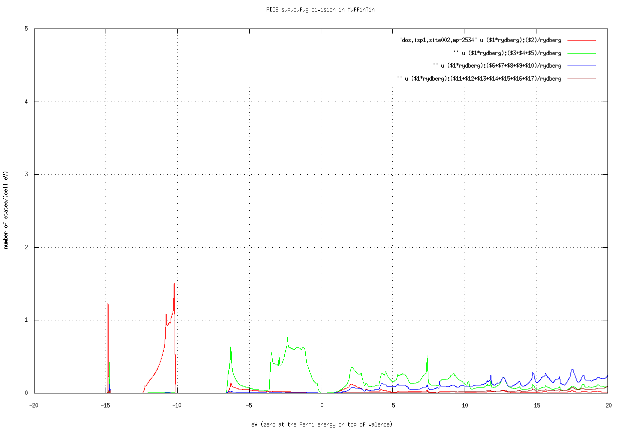alt text .This is PDOS at As site of mp-2534. Be careful about the number of k points. You may need to enlarge number of k points for accurate DOS,PDOS. Then use -vnk1=10 -vnk2=10 -vnk3=10 as the option, such as job_tdos mp-2534 -np 8 -vnk1=10 -vnk2=10 -vnk3=10. Check it by grep BZ_NKABC llmf_tdos and look into save.mp-2534.

Step 4. Create k-path and Brillouin zone for band plot

After lmf converges, make a band plot with job_band explained later on. The normality of the calculation of bands can be confirmed by the band plot (for magnetic systems, check the total magnetic moment and the magnetic moment for each site).

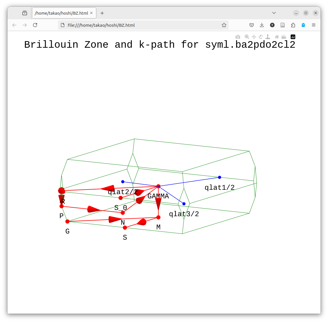
Before job_band, run getsyml gaas. Install any missing packages with pip. It is on spglib by Togo and seekpath. After finished, view BZ.html. It shows the k-path in the BZ. We show an example for ba2pdo2cl2 in the figure below. It is an interactive figure written with plotly, so you can read the coordinate values.

getsyml foobar

(foobar is that in ctrl.foobar)

Samples of BZ.html by getsyml are seen at https://ecalj.sakura.ne.jp/BZgetsyml/

Step 5. band plot

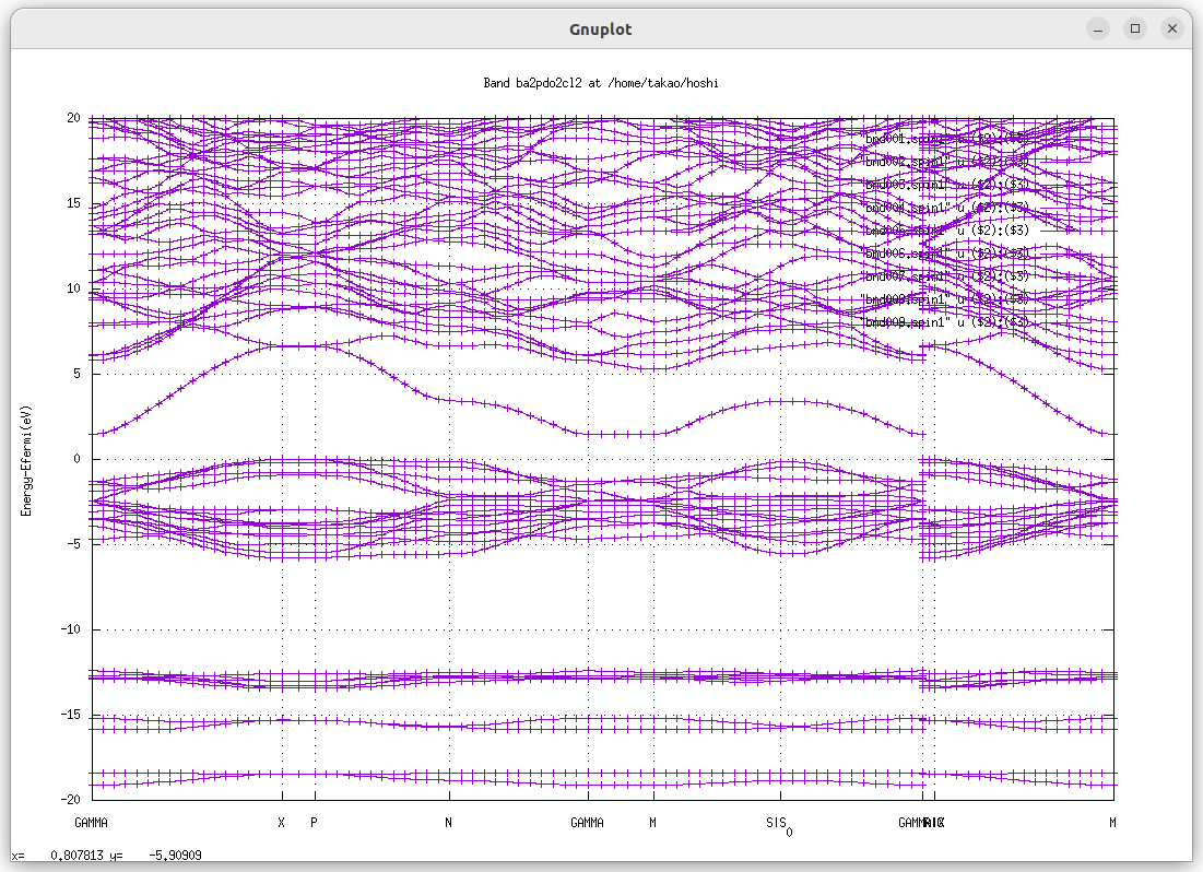
（this is a case for ba2pdo2cl2 ）

>job_band ctrl.ba2pdo2cl2 -np 8

A gnuplot script can be created. Edit it if necessary. If you edit syml.ba2pdo2cl2 before job_band, you can adjust the symmetry line and mesh size.

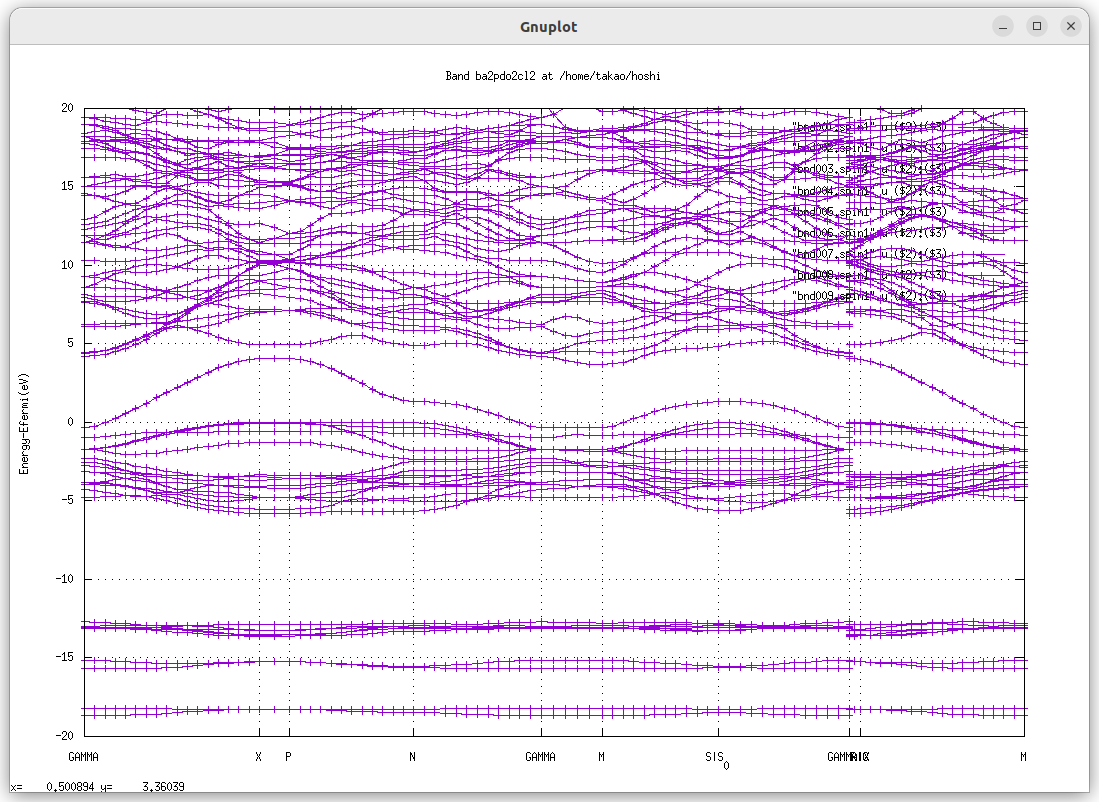
The following picture is the LDA bands for the default calculation of ba2pdo2cl2 (the names of the symmetric points can be confirmed with BZ.html. In addition, look into syml.foobar). 0 eV is the Fermi energy. Since this is metallic, we see no band gap. .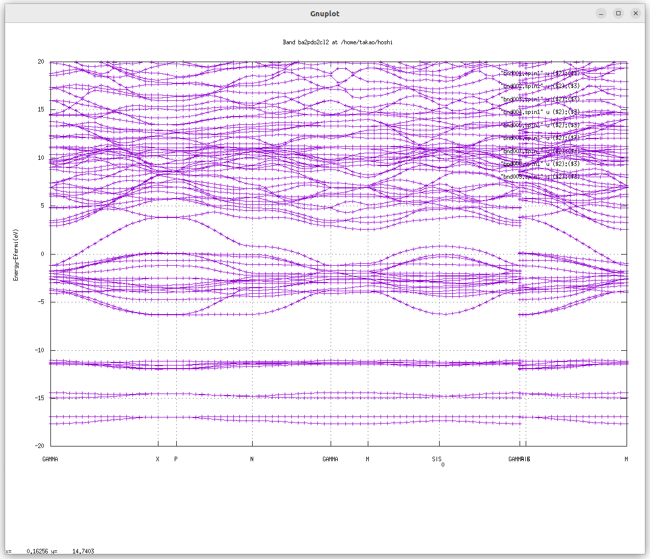

Here we are talking about band energies.

In ecalj, the k mesh for lmf (ctrl) and the k mesh for GW (n1n2n3 specified in GWinput) can be different. The former has affected little on computational time, but the latter has a large effect (thus we want to reduce n1n2n3 in GWinput).
In ecalj's band plot mode, theoretically degenerated bands because of symmetry at the BZ edge are not degenerated. This is because there are limited numbers of APW basis functions, so run the band plot with pwemax=4, etc. (Temporary solution: We want to automate it).

job_tdos, job_fermisurface, job_pdos

job_pdos calculates PDOS, job_tdos calculates total DOS, and job_fermisurface draws the Fermi surface with Xcrysden. job_fermisurface can be used to draw the shape of the CBM bottom as ellipsoid of Si. xxx

Step 6. QSGW calculation

We now run QSGW calculations. QSGW is computationally very expensive. So we recommend you to run smaller systems at first.

For QSGW calculations, we need one additional input file GWinput, whose template is generated by mkGWinput.

mkGWinput ctrl.mp-2534

Then copy and edit GWimput.tmp to GWinput.

In GWinput, n1n2n3 should be smaller than nk1 nk2 nk3 in ctrl usually, in order to reduce computational time (1/2 or 2/3 of ctrl, for example) If n1n2n3 6 6 6 for Si, it is good. Except k points, not need to modify so much (ask us). GWinput is explained here. Input system is different from ctrl. Here is a convergence behavior of the band gap for GaAs taken from Ref.[3], 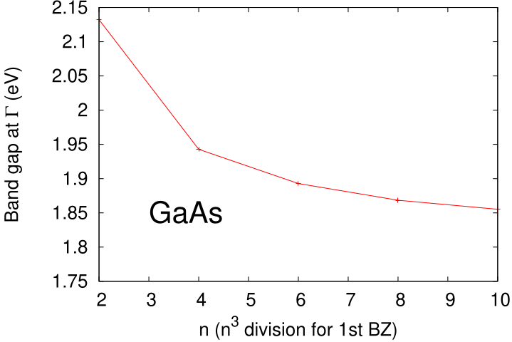convGaAs From this picture, I may say 4 4 4 is not so bad if we assume ~0.1eV accuracy. 6 6 6 is good. More than 8 8 8 is for numerical check(not fruitful for practical applications).

Flow of QSGW calculation with the script gwsc

We run the QSGW calculations with gwsc. For semiconductors, several QSGW iterations are fine, close enough to final results. QSGW is to obtain band structures (or one-body Hamiltonian), the total energy is not yet.

QPU file contains diagonal components of GW calculations. Note that our Mixed Produce basis is a key technology for the GW calculation.

gwsc -np NP [--phispinsym] [--gpu] [--mp] nloop extension

(--phispinsym is for magnetic materials to keep the same basis for up and down)

Then console outputs of gwsc is somthing like

### START gwsc: ITERADD= 1, MPI size=  4, 4 TARGET= si
===== Ititial band structure ====== 
---> No sigm. LDA caculation for eigenfunctions 
0:00:00.226245   mpirun -np 1 /home/takao/bin/lmfa si     >llmfa
0:00:00.807062   mpirun -np 4 /home/takao/bin/lmf  si     >llmf_lda
===== QSGW iteration start iter 1 ===
0:00:03.071054   mpirun -np 1 /home/takao/bin/lmf si     --jobgw=0 >llmfgw00
0:00:03.904403   mpirun -np 1 /home/takao/bin/qg4gw    --job=1 > lqg4gw
0:00:04.431022   mpirun -np 4 /home/takao/bin/lmf si     --jobgw=1 >llmfgw01
0:00:05.918216   mpirun -np 1 /home/takao/bin/heftet --job=1    > leftet
0:00:06.444439   mpirun -np 1 /home/takao/bin/hbasfp0 --job=3    >lbasC
0:00:07.064558   mpirun -np 4 /home/takao/bin/hvccfp0 --job=3    > lvccC
0:00:07.812283   mpirun -np 4 /home/takao/bin/hsfp0_sc --job=3    >lsxC
0:00:08.545956   mpirun -np 1 /home/takao/bin/hbasfp0 --job=0    > lbas
0:00:09.156775   mpirun -np 4 /home/takao/bin/hvccfp0 --job=0    > lvcc
0:00:09.884064   mpirun -np 4 /home/takao/bin/hsfp0_sc --job=1    >lsx
0:00:10.644292   mpirun -np 4 /home/takao/bin/hrcxq   > lrcxq
0:00:11.482931   mpirun -np 4 /home/takao/bin/hsfp0_sc --job=2    > lsc
0:00:12.460776   mpirun -np 1 /home/takao/bin/hqpe_sc    > lqpe
0:00:13.019735   mpirun -np 4 /home/takao/bin/lmf si     >llmf
===== QSGW iteration end   iter 1 ===
OK! ==== All calclation finished for  gwsc ====

...

The console outputs are redirected to log files l*. lsxC is the exchange self-energy due to cores. lsx is for exchange. lsc is correlation. lvcc is for Coulomb matrix。 In this calculation we run gwsc -np 8 1 si, where 1 is the number of QSGW iteration. If you repeat gwsc, we have additional QSGW iterations on top the previous calculations.

a case of La2CuO4

For La2CuO4, I had

2025-06-27 19:09:01.465241   mpirun -np 1 echo --- Start gwsc ---
--- Start gwsc ---
option=   -vssig=0.8 
### START gwsc: ITERADD= 5, MPI size=  32, 32 TARGET= lcuo
===== Ititial band structure ====== 
---> We use existing sigm file
0:00:00.041902   mpirun -np 32 /home/takao/bin/lmf lcuo   -vssig=0.8  >llmf_start
We found QPU.5 -->start to generate QPU.6...
===== QSGW iteration start iter 6 ===
0:00:18.111042   mpirun -np 1 /home/takao/bin/lmf lcuo   -vssig=0.8  --jobgw=0 >llmfgw00
0:00:18.233440   mpirun -np 1 /home/takao/bin/qg4gw   -vssig=0.8 --job=1 > lqg4gw
0:00:18.488197   mpirun -np 32 /home/takao/bin/lmf lcuo   -vssig=0.8  --jobgw=1 >llmfgw01
0:00:40.910973   mpirun -np 1 /home/takao/bin/heftet --job=1   -vssig=0.8 > leftet
0:00:41.052760   mpirun -np 1 /home/takao/bin/hbasfp0 --job=3   -vssig=0.8 >lbasC
0:00:43.290214   mpirun -np 32 /home/takao/bin/hvccfp0 --job=3   -vssig=0.8 > lvccC
0:01:00.327823   mpirun -np 32 /home/takao/bin/hsfp0_sc --job=3   -vssig=0.8 >lsxC
0:01:45.547149   mpirun -np 1 /home/takao/bin/hbasfp0 --job=0   -vssig=0.8 > lbas
0:01:46.806858   mpirun -np 32 /home/takao/bin/hvccfp0 --job=0   -vssig=0.8 > lvcc
0:01:59.034735   mpirun -np 32 /home/takao/bin/hsfp0_sc --job=1   -vssig=0.8 >lsx
0:02:45.526614   mpirun -np 32 /home/takao/bin/hrcxq  -vssig=0.8 > lrcxq
0:06:51.996781   mpirun -np 32 /home/takao/bin/hsfp0_sc --job=2   -vssig=0.8 > lsc
0:23:31.022636   mpirun -np 1 /home/takao/bin/hqpe_sc   -vssig=0.8 > lqpe
0:23:33.062303   mpirun -np 32 /home/takao/bin/lmf lcuo   -vssig=0.8  >llmf
===== QSGW iteration end   iter 6 ======== QSGW iteration start iter 7 ===
0:24:12.969096   mpirun -np 1 /home/takao/bin/lmf lcuo   -vssig=0.8  --jobgw=0 >llmfgw00
...

This is without GPU. We see one QSGW iteration requires 24 minutes (start timing is shown at the top of lines). Since I had 5th-QSGW iteration finished (checked by the existence of QPU.5run), it start from 6th iteration.

a case study of ba2pdo2cl2.

Run

mkGWinput ba2pdo2cl2

to generate GWinput.tmp, which is a setting file for QSGW. After copying this to GWinput, you may need to edit GWinput. Minimum thing to edit is the number of k points for the self energy (n1n2n3). Compared with k points in ctrl (nk1,nk2,nk3), we use small numbers. (We often use 1/2 or 2/3 of k points given in ctrl as nk1,nk2,nk3).

There are another setting in GWinput. However, we usually do not need to touch things except n1n2n3 if you treat non-magnetic semiconductors.

Then you can run QSGW calculation with

gwsc -np 32 1 ba2pdo2cl2

. Here 1 means the number of QSGW iterations. QSGW iteration is quite time-consuming. gwsc gives minimum help (we need to explain options elsewhere).

The iteration is kept in rst.foobar:electron density, sigm.*:vxcqsgw. (Remove these files in addition to *run files/directories if you like to start from the beginning).

It requires 53 minutes to run one iteration of QSGW.
job_band ba2pdo2cl2 -np 32 gives the following picture. QSGW one-shot changes band structure around Ef from that in LDA.But still metallic, no band gaps.
To continue QSGW iteration, run

gwsc -np 32 nx ba2pdo2cl2

Since you did 1 already. You will have the results of 1+nx QSGQ iteration.

when we run 8 iterations as for ba2pdo2cl2, we had band gap 2.1 eV. We saw band gap after 4th iteration.
For comparison with experiments, we recommend to use ssig=0.8 (set in ctrl.foobar file), which is called as QSGW80.
Spin-orbit coupling. After you obtain sigm.foobar, you set SO=1 (LdotS scheme) and run lmf. Then you can include effect of SOC. Sinc SO=1 is not implemented in the whole gwsc cycle, we have to include SOC just at the end step (We include SOC after we fix VxcQSGW).
If you run

gwsc -np 32 5 ba2pdo2cl2 -vssig=0.8

, this overide ssig, which is defined in ctrl.ba2pdo2cl2, in lmf calculations. (Check it in save.ba2pdo2cl2)

a case of KTaO3

Example of QSGW for KTaO3 (perovskite,mp-3614）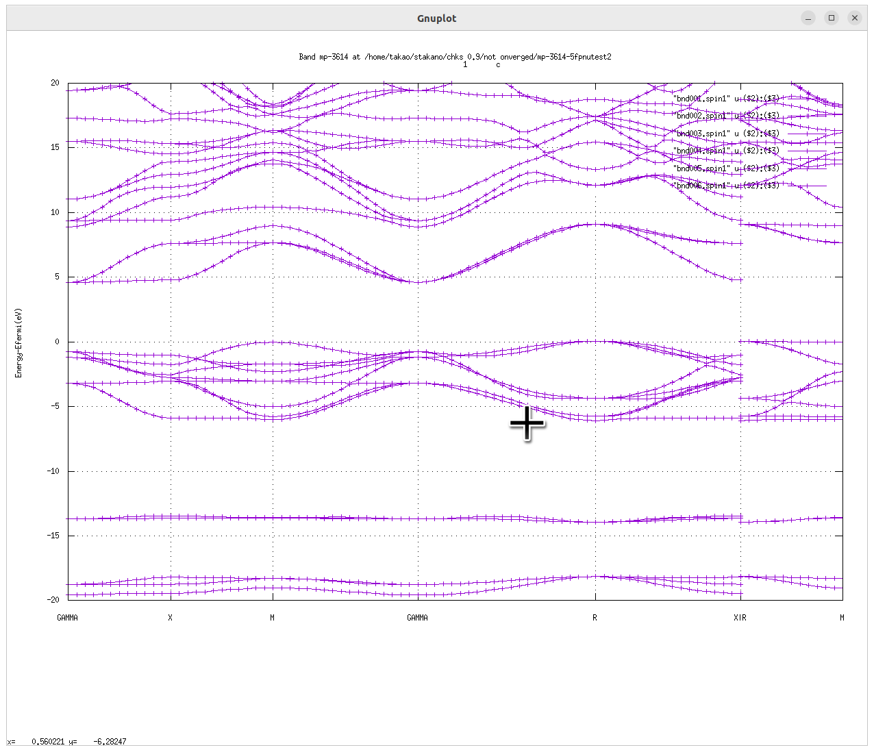

lmchk

lmchk mp-2534

is to check the crystal symmetry. In addition determine MT radius. and Check the ovarlap of MTs. Defaults setting is with -3% overlap.(no overlap).

symmetry
MT overlap If you have less symmetry rather than the symmetry of lattice for magnetic systems, you have to set crystal symmetry by hand.

This can be done by adding space group symmetry generator to SYMGRP (instead of find). We need to pay attention for this point in the case of SOC.

how to write space-group operation

For example r3x means 3-fold axis along x. How to express space-group operations in ecalj are explained at SYMGRP section at lmf.md.

How to start over calcualtions

Remove mix* rst* (mix* is mixing files) If MT radius are changed, start over from lmfa (remove atm* files)

As long as converged, no problem.
If you have 3d spagetti-like entangled bands at Ef, need caution.

jobmaterials.py: mini database for computational tests

At ecalj/MATERIALS/, type ./jobmaterials.py. It shows a help with a list of materials. It contains samples of simple materials. It performs LDA calculations and generates GWinput for materials. (I think MATERIALS/ is not organaized well. We are going to clean up)

How to run

./job_materials.py

gives a help, showing a list of materials as

 === Materials in Materials.ctrls.database are:===
 2hSiC 3cSiC 4hSiC AlAs AlN AlNzb AlP AlSb Bi2Te3 C
 CdO CdS CdSe CdTe Ce Cu Fe GaAs GaAs_so GaN
 GaNzb GaP GaSb Ge HfO2 HgO HgS HgSe HgTe InAs
 InN InNzb InP InSb LaGaO3 Li MgO MgS MgSe MgTe
 Ni NiO PbS PbTe Si SiO2c Sn SrTiO3 SrVO3 YMn2
 ZnO ZnS ZnSe ZnTe ZrO2 wCdS wZnS

Run Si for example:

./job_materials.py Si

performs LDA calculation of Si at ecalj/MATERIALS/Si/. '--all' works as well instead of 'Si'.

job_materials.py works as follows for given names. Step 1. Generate ctrls.* file for Materials.ctrls.database. (names are in DATASECTION:) Step 2. Generate ctrl by ctrlgenM1.py Step 3. Make directtory such as Si/ and copy ctrls.si ctrl.si and GWinput (this is for QSGW) Step 4. run lmfa and lmf We can skip step 4 with --noexec. Run "job_materials --all --noexec" is an idea to generate all input files for materials in the database. Watch no strange erros appear.

Key input files are ctrls.si,ctrl.si . See sections below. rst.si contains self-consistent electron density. Check iterations with the output file save.si. The console output of lmf is in llmf. Not need to know all the console outputs.
Before QSGW, it is better to confirm the LDA level calculations are fine. In order to do the confirmation, band plot is convenient. For band plot we need the symmetry line as syml.si which can be generated by
```
getsyml si
```
Then run
```
job_band si -np 8
```
results band plots in the gnuplot.

This is the end of GetStarted. Goto UsageDetailed

ecalj MainDocument ​

Licence ​

Install ​

Features of ecalj package ​

Overview of QSGW ​

GetStarted ​

Step 0. Get POSCAR ​

Step 1. convert POSCAR to ctrls ​

Step 2. Get ctrl from ctrls ​

Install VESTA ​

Step 3. LDA calculation ​

job_tdos, job_pdos ​

Step 4. Create k-path and Brillouin zone for band plot ​

Step 5. band plot ​

job_tdos, job_fermisurface, job_pdos ​

Step 6. QSGW calculation ​

Flow of QSGW calculation with the script gwsc ​

a case of La2CuO4 ​

a case study of ba2pdo2cl2. ​

a case of KTaO3 ​

lmchk ​

how to write space-group operation ​

How to start over calcualtions ​

jobmaterials.py: mini database for computational tests ​

ecalj MainDocument

Licence

Install

Features of ecalj package

Overview of QSGW

GetStarted

Step 0. Get POSCAR

Step 1. convert POSCAR to ctrls

Step 2. Get ctrl from ctrls

Install VESTA

Step 3. LDA calculation

job_tdos, job_pdos

Step 4. Create k-path and Brillouin zone for band plot

Step 5. band plot

job_tdos, job_fermisurface, job_pdos

Step 6. QSGW calculation

Flow of QSGW calculation with the script gwsc

a case of La2CuO4

a case study of ba2pdo2cl2.

a case of KTaO3

lmchk

how to write space-group operation

How to start over calcualtions

jobmaterials.py: mini database for computational tests